The WeChat public account on quantitative investment and machine learning is a mainstream self-media in the industry, focusing on fields such as quantitative investment, hedge funds, Fintech, artificial intelligence, and big data. The public account has over 300K+ followers from industries such as public offerings, private equity, securities, futures, banks, insurance, and universities, and has won the AMMA Excellent Brand Power and Excellent Insight Awards, being named “Best Author of the Year” by Tencent Cloud + Community for four consecutive years.
Title: Time Series Forecasting with Transformer Models and Application to Asset Management
Authors: Edmond LEZMI, Jiali XU
The development of deep learning provides us with powerful tools to create the next generation of time series forecasting models. Deep artificial neural networks, as a fully data-driven approach to learning temporal dynamics, are particularly well-suited for the challenge of finding complex nonlinear relationships between inputs and outputs. Initially, recurrent neural networks and their extended LSTM networks were designed to handle sequential information in time series. Then, convolutional neural networks were used for time series forecasting due to their success in image analysis tasks.
The Transformer model was subsequently released by Google in 2017 (Vaswani et al., 2017) and was designed to use attention mechanisms to process sequential data, addressing sequence learning problems in natural language processing (such as machine translation). Essentially, the Transformer model allows us to transform an input sequence from one domain into an output sequence in another domain. For example, we can train a Transformer model to translate English sentences into French. To draw an analogy, if we view a segment of a time series as a sentence in one language and the following segment as a sentence in another language, then this multi-step time series forecasting problem is also a sequence learning problem. Therefore, Transformer models can also be used to address forecasting problems in time series analysis. As noted by Wen et al. (2022), many variants of the Transformer model have been successfully applied to time series forecasting tasks, such as Li et al. (2019) and Zhou et al. (2021). With the introduction of the Transformer model architecture, the application of deep learning in time series forecasting has become increasingly widespread. To address the challenges present in time series forecasting, more and more Transformer architectures have been proposed, such as Temporal Fusion Transformers, Informer, Autoformer, and Crossformer.
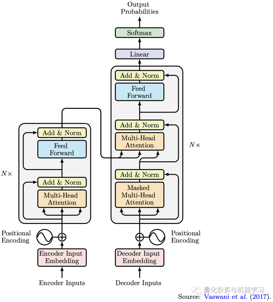 The Transformer model employs a seq2seq architecture, whose flexibility allows us to tackle more complex sequence learning problems.By leveraging attention mechanisms, we can capture long-term dependencies between elements in a sequence, especially using multi-head attention to capture information in the sequence from different perspectives. Additionally, apart from the self-attention mechanism we apply to the encoder and decoder, we also use another attention mechanism to capture the correlation between the encoder and decoder. Since the self-attention mechanism does not analyze their inputs in chronological order, Transformer models are less likely to be affected by vanishing or exploding gradient problems.Another advantage of Transformer models is their parallelization. Because of the multi-head attention mechanism, each head in the Transformer model can capture relationships between elements in the input across different criteria. In contrast, RNN models require data to be input sequentially in chronological order, which makes them unable to parallelize.
By understanding the principles of the attention mechanism in Transformer models and the seq2seq architecture, we can apply these advanced machine learning techniques to time series forecasting, particularly for multi-step multivariate time series forecasting, as illustrated in the following diagram. In such tasks, we need to learn temporal relationships in the time series to model the evolution of dynamic systems, as well as learn spatial relationships in multivariate data to understand how they influence each other. In the financial sector, time series forecasting is a common task.
In financial time series forecasting, there are generally two types of application scenarios:
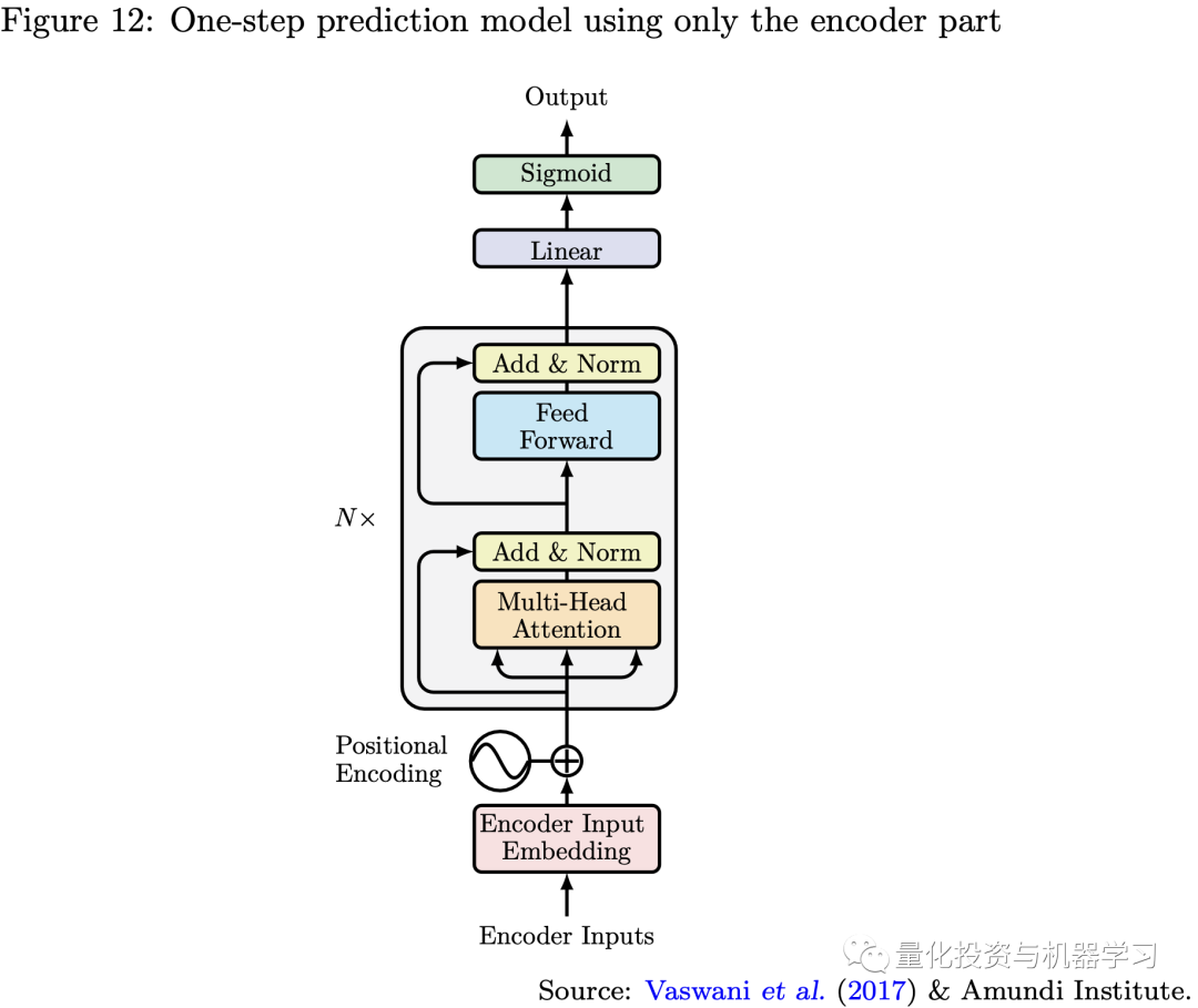
Single-step Forecasting Using Only the Encoder
As illustrated below, if we only use the encoder part of the Transformer model and connect the encoder output directly to the last layer, the model resembles a traditional RNN’s many-to-one forecasting but employs self-attention mechanisms. Thus, we can use this model for single-step forecasting, just as we often use recursive models like RNNs or LSTMs, which can be completely replaced by the encoder due to its flexible parallelization, more effective long-term memory, and fewer vanishing or exploding gradient problems. We can also handle different problems, such as classification or regression, by modifying the activation function of the model’s last layer.
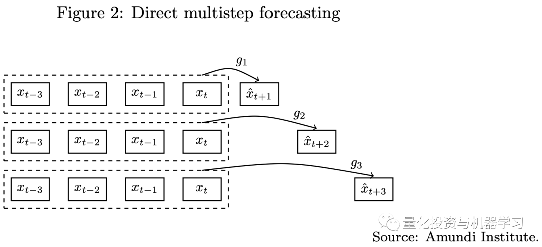
Multi-step Forecasting Using the Full Model (Encoder and Decoder)
Traditional multi-step forecasting has two approaches, including iterative and direct forecasting (as shown in the diagram below). Whether using iterative or direct methods, single-step forecasting models are challenging to apply to multi-step forecasting tasks. Due to the seq2seq architecture in Transformer models, we can use these models to handle multi-step forecasting problems.
The Transformer model employs a seq2seq architecture, whose flexibility allows us to tackle more complex sequence learning problems.By leveraging attention mechanisms, we can capture long-term dependencies between elements in a sequence, especially using multi-head attention to capture information in the sequence from different perspectives. Additionally, apart from the self-attention mechanism we apply to the encoder and decoder, we also use another attention mechanism to capture the correlation between the encoder and decoder. Since the self-attention mechanism does not analyze their inputs in chronological order, Transformer models are less likely to be affected by vanishing or exploding gradient problems.Another advantage of Transformer models is their parallelization. Because of the multi-head attention mechanism, each head in the Transformer model can capture relationships between elements in the input across different criteria. In contrast, RNN models require data to be input sequentially in chronological order, which makes them unable to parallelize.
By understanding the principles of the attention mechanism in Transformer models and the seq2seq architecture, we can apply these advanced machine learning techniques to time series forecasting, particularly for multi-step multivariate time series forecasting, as illustrated in the following diagram. In such tasks, we need to learn temporal relationships in the time series to model the evolution of dynamic systems, as well as learn spatial relationships in multivariate data to understand how they influence each other. In the financial sector, time series forecasting is a common task.
In financial time series forecasting, there are generally two types of application scenarios:
Single-step Forecasting Using Only the Encoder
As illustrated below, if we only use the encoder part of the Transformer model and connect the encoder output directly to the last layer, the model resembles a traditional RNN’s many-to-one forecasting but employs self-attention mechanisms. Thus, we can use this model for single-step forecasting, just as we often use recursive models like RNNs or LSTMs, which can be completely replaced by the encoder due to its flexible parallelization, more effective long-term memory, and fewer vanishing or exploding gradient problems. We can also handle different problems, such as classification or regression, by modifying the activation function of the model’s last layer.
Multi-step Forecasting Using the Full Model (Encoder and Decoder)
Traditional multi-step forecasting has two approaches, including iterative and direct forecasting (as shown in the diagram below). Whether using iterative or direct methods, single-step forecasting models are challenging to apply to multi-step forecasting tasks. Due to the seq2seq architecture in Transformer models, we can use these models to handle multi-step forecasting problems.
Challenges in Financial Time Series Forecasting
In the investment field, one of the most challenging and crucial tasks in portfolio construction is predicting future returns. We also believe that machine learning models may provide some computational advantages for quantitative investment, such as the ability to capture nonlinear relationships and temporal dependencies. For instance, Cherief et al. (2022) used tree-based machine learning algorithms to capture nonlinearity and detect interdependencies among risk factors in the Euro and USD credit space.
However, we believe that the successful application of machine learning models requires meeting many conditions:Data must be clean, the volume of data must be sufficient, patterns presented in the data must be persistent, model complexity must be appropriate, and the quality of training must be very good.
In practice, due to the differences between financial time series data and data from other fields like text or images, we often cannot meet all the above conditions. The main issues are:
Low Signal-to-Noise Ratio
Unlike traditional machine learning use cases such as image processing or natural language processing, the signal-to-noise ratio in financial data is very low. In other words, there is too much noise in the data, making the system less predictable. It is worth noting that if we consider a classification or regression problem, noise exists not only in the features but also in the labels. For example, we can view the returns of an asset as the sum of expected returns and noise. We can easily observe realized returns from market data, but knowing what the true expected return is can be very challenging, especially in the presence of significant noise.
Markets are Ever-Changing
This is why the term “Regime Shift” is used to describe changes in the interconnections between various components of the financial system. A classic example is using expansion or recession to describe different mechanisms of the economic cycle and bull or bear markets to describe cycles in financial markets. To train a robust machine learning model, apart from ensuring that the training and validation datasets have similar distributions, we must also ensure that future data follows the same distribution. For most financial data, achieving these two points is very challenging. Therefore, if we want to have a machine learning model that can adapt to the current regime, the input used for training the model should not include data that is too old.
Limited Data in the Financial Industry
The primary issue is that all financial data is random and non-stationary, making it difficult to generate new data through experiments that track the temporal dynamics of financial markets. Additionally, scale limitations arise not only from features but often from labels, as we prefer to directly predict the returns of financial assets with limited observations. For instance, if we have 20 years of daily returns for a financial asset, we only have about 5000 data points distributed across different market regimes. For extreme events, the occurrences are much lower, such as during financial crises or the COVID-19 pandemic. This magnitude of data is insufficient relative to the number of parameters to train a deep learning model, especially in multivariate cases. Therefore, aside from the reasons mentioned in the previous paragraph, the capacity of the dataset used for training models is often limited.
How to Balance Model Complexity
When we use machine learning techniques in quantitative investment, especially when classifying or regressing asset returns, we often input all features into a complex deep learning model, hoping to capture nonlinear relationships and complex structures in financial data.Based on the three issues we previously mentioned regarding machine learning applications in finance, we easily make two mistakes:
1. Due to the quality and quantity of data in the financial field being inferior to many other areas using machine learning techniques, the model’s accuracy will not be high enough to determine whether the model is good and robust. In particular, the labels we use for machine learning, such as the positive and negative signs of asset returns, are very unstable, noisy, and sometimes erroneous. Therefore, using these low-quality labels with complex models will lead to models yielding no results or overfitting.
2. Based on our experience, we find that using complex deep learning models without sufficient data for training tends to emphasize certain features, which means the model often overfits. In this case, we face the issue of losing diversification, which is one of the most critical aspects of quantitative investment.
Therefore, when we cannot significantly improve model accuracy, using complex deep learning models with many features often results in lower out-of-sample performance than traditional rule-based models, as in trying to capture more complex relationships in the data, we similarly lose opportunities for diversification.Hence, we believe that we should choose a balance between model complexity and diversification. Inspired by the concept of weak learners in ensemble learning, we tend to train many structurally simple weak models in practice. Then, we aggregate the predictions of all models to build a strong model, rather than just training a complex machine learning model. Additionally, we select different types of weak models because we want them to obtain useful information from different aspects. When training various weak models, we should use parameters/hyperparameters as sparingly as possible to avoid overfitting, while using different sets of hyperparameters to achieve more robust results. Another advantage of training models with fewer features is that, even with a relatively small amount of data, we can train models well, even using neural network structures.
Building very complex machine learning models using data from the financial sector is extremely challenging because the data used to train the models contains many flaws.Therefore, our goal is to sacrifice model complexity for better calibration and prediction quality, meaning that the model fits financial data more easily, resulting in lower out-of-sample errors.We believe this is a very suitable solution for the application of machine learning in quantitative investment, where the quality and quantity of data are relatively low compared to other industries, and we cannot find a clear pattern to comprehensively describe actions in the market. The sacrifice of model complexity will be compensated by diversification in quantitative investment. Therefore, when we want to apply traditional machine learning models or deep learning models to predict future asset returns, we prefer to use low-complexity models with simple structures and fewer features, such as Transformer models, which have shallower encoder and decoder parts, using two to three features as input. In this case, using deep learning models is still to leverage their ability to handle time series and capture long-term memory in the data, rather than their ability to fit complex nonlinear relationships with very deep structures.
This approach, based on maintaining the principle of diversification, aligns with the Vapnik-Chervonenkis theory, which attempts to provide a statistical explanation for the learning process. According to Vapnik (2000), when training machine learning models, we need to find a balance between model complexity, calibration quality, and prediction quality. In the context of deep learning, model complexity refers to the number of parameters used in the model, such as the number of layers in a neural network and the number of nodes per layer. More parameters mean a more complex model that can learn more complex relationships in the data, but requires more data for model calibration during training. Calibration quality is measured based on training error and model complexity; to improve calibration quality, data must match each other. For example, overly simple models cannot capture all the information in the data, linear models cannot find nonlinear relationships in the training dataset, and overly complex models require large amounts of high-quality data for training, which is often impossible. Prediction quality relates to the model’s out-of-sample error, with complex models often prone to overfitting, leading to larger out-of-sample errors.
Case Studies of Transformer in Quantitative Investment
Case 1: Trend Following Strategy (Single-step Forecasting)
We first look at a case of single-step forecasting. In the case of trend-following strategy, we will use the encoder part of the Transformer model to predict the signs of asset returns for the next week using short-term, medium-term, and long-term trends of the asset.In our example, we do not train a complex model by putting all these features together. We borrowed the idea of weak learners from ensemble learning, and we will train many models, each simple, using only one or two features. Finally, we will aggregate these weak learners into a strong learner.
We apply logistic regression, support vector machines, and encoders with attention mechanisms to classify the excess returns of each asset for the next week (which is a classification model). For each model, we train weak learners using one or two features and aggregate the results of all weak learners to build a strong learner. To avoid selection bias, we calculate the short-term, medium-term, and long-term returns of assets using five classic backtesting windows (1 month, 2 months, 3 months, 6 months, 12 months) as the feature set for the model.
The purpose of this backtest is to illustrate the importance of balancing model complexity and diversification when applying machine learning models to quantitative investment, and to test whether machine learning models can capture more information in the data. We use different models to obtain information from different aspects of the data:
1. The benchmark strategy is equivalent to a linear classifier, training on only one feature, such as 12-month momentum, with a threshold set at 0.9.
2. Logistic regression also establishes a linear classifier trained on only one feature, but the threshold is learned from the data.
3. To capture nonlinear relationships in the data using the RBF kernel (Radial Basis Function kernel) in support vector machines, we train a model using two features at a time, such as 1-month and 12-month momentum. When we have five features, we must train ten models.
4. We also trained the encoder with a multi-head attention mechanism to capture information in the time series dimensions. The features used to calibrate the model remain the trends using five different backtesting windows, but these features are input into the model as time series. We will apply the same idea as before, with each model also using two features for training.
For each model, if we need to select hyperparameters for the model, we will choose a set of hyperparameters rather than just one, and average the predictions from all models using different hyperparameters. For the encoder using the multi-head attention mechanism, we adopted a simple structure with two encoder blocks; since our design is to use a small number of features as input to train the model, this linear layer does not need to have too many nodes.
In the backtest, we used weekly rebalancing and set the trading cost for futures at 2 bps. We recalibrated the machine learning models every three months based on the past three years of observational data. Due to the random effects during the model training process, we train multiple models on the same training dataset at each recalibration date, and then average the predictions from all models. Below are the backtesting results for different types of models:
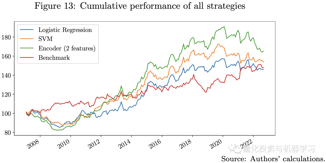
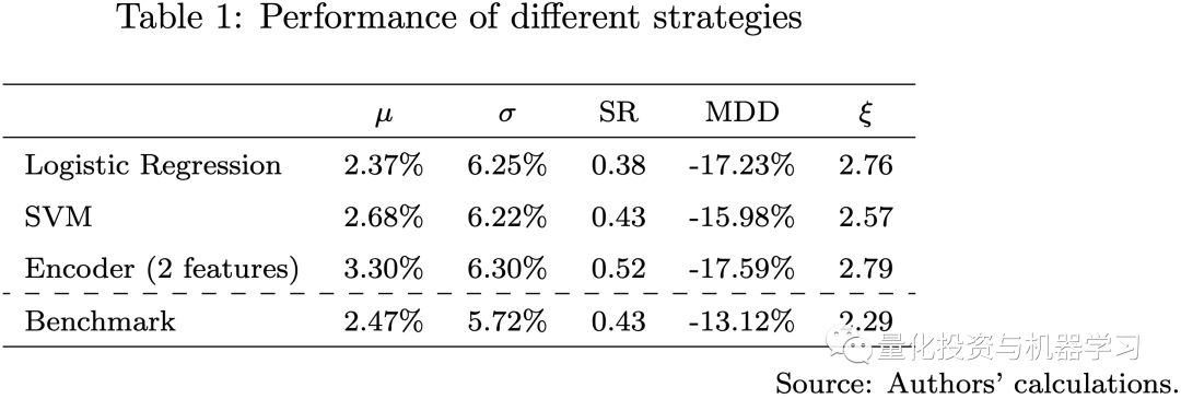 From the above figures, we note that all strategies using machine learning models perform significantly differently compared to the benchmark strategy. The Sharpe ratios of the logistic regression and SVM models are comparable to the benchmark strategy, while the encoder with multi-head attention outperforms all other models.All strategies exhibit the same level of volatility and maximum drawdown. Our three machine learning models have different levels of model complexity and use different numbers of features for training. In this regard, the more complex the model, the more likely it is to capture useful information in the data. We observed in the backtest that after 2020, all machine learning models struggled; during this period, COVID-19, high inflation, interest rate hikes, the high correlation between stocks and bonds, and the Russia-Ukraine war made financial markets different from any time before.
Due to larger out-of-sample errors, the more complex the model, the worse the performance during this period. This is why the performance of the encoder model declined rapidly after 2021. In this case, a feasible option is to increase the frequency of model recalibration and use more recent data during training to quickly adapt to actual market conditions.The backtest results indicate that using machine learning models can capture more useful information in the data to predict future returns; thus, we can try to enhance the strategy by adding some macro factors into the model.
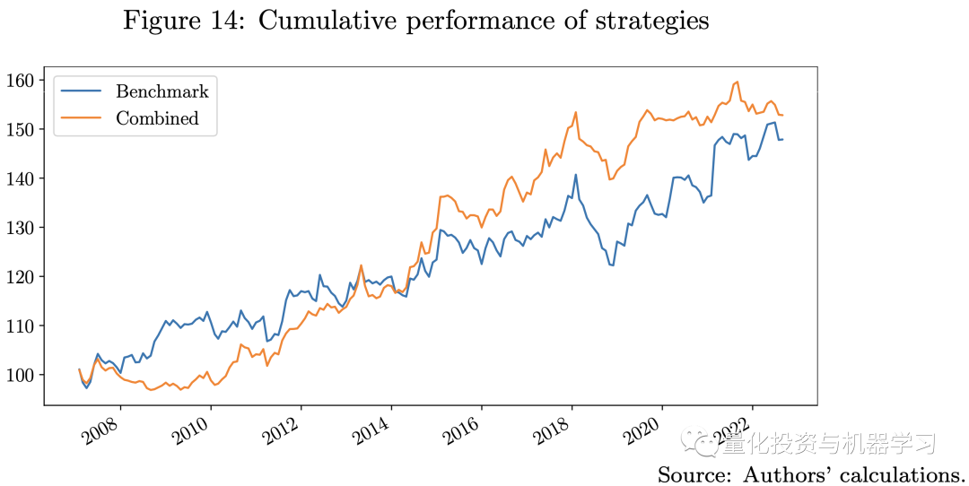
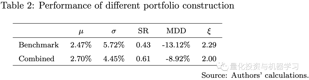
In the following diagram, we compare the benchmark strategy with the ensemble strategy, the ensemble strategy combines three machine learning strategies and the benchmark strategy, using a risk parity approach. The performance of the ensemble strategy surpasses that of the benchmark strategy, with a higher Sharpe ratio and lower maximum drawdown. This result suggests that machine learning models may offer some computational advantages in quantitative investment.It particularly confirms the key idea of our strategy design, which is to train many weak machine learning models to build strong learners, ensuring a balance between model complexity and maintaining diversification.
Case 2: Portfolio Optimization (Multi-step Forecasting)
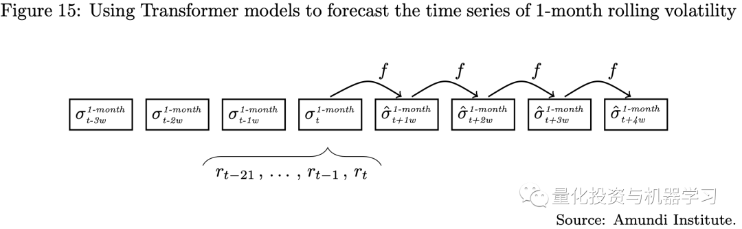
For the multi-period portfolio optimization problem, we will use the full Transformer model to perform multi-period forecasting of volatility time series and use these forecasts as inputs for portfolio allocation methods such as mean-variance optimization and risk budgeting methods. We will compare the differences between single-period optimal portfolios, multi-period optimal portfolios based on historical estimates, and multi-period optimal portfolios based on Transformer predictions.
From the above figures, we note that all strategies using machine learning models perform significantly differently compared to the benchmark strategy. The Sharpe ratios of the logistic regression and SVM models are comparable to the benchmark strategy, while the encoder with multi-head attention outperforms all other models.All strategies exhibit the same level of volatility and maximum drawdown. Our three machine learning models have different levels of model complexity and use different numbers of features for training. In this regard, the more complex the model, the more likely it is to capture useful information in the data. We observed in the backtest that after 2020, all machine learning models struggled; during this period, COVID-19, high inflation, interest rate hikes, the high correlation between stocks and bonds, and the Russia-Ukraine war made financial markets different from any time before.
Due to larger out-of-sample errors, the more complex the model, the worse the performance during this period. This is why the performance of the encoder model declined rapidly after 2021. In this case, a feasible option is to increase the frequency of model recalibration and use more recent data during training to quickly adapt to actual market conditions.The backtest results indicate that using machine learning models can capture more useful information in the data to predict future returns; thus, we can try to enhance the strategy by adding some macro factors into the model.
In the following diagram, we compare the benchmark strategy with the ensemble strategy, the ensemble strategy combines three machine learning strategies and the benchmark strategy, using a risk parity approach. The performance of the ensemble strategy surpasses that of the benchmark strategy, with a higher Sharpe ratio and lower maximum drawdown. This result suggests that machine learning models may offer some computational advantages in quantitative investment.It particularly confirms the key idea of our strategy design, which is to train many weak machine learning models to build strong learners, ensuring a balance between model complexity and maintaining diversification.
Case 2: Portfolio Optimization (Multi-step Forecasting)
For the multi-period portfolio optimization problem, we will use the full Transformer model to perform multi-period forecasting of volatility time series and use these forecasts as inputs for portfolio allocation methods such as mean-variance optimization and risk budgeting methods. We will compare the differences between single-period optimal portfolios, multi-period optimal portfolios based on historical estimates, and multi-period optimal portfolios based on Transformer predictions.
For multi-period portfolio optimization, the goal is to maximize utility over the next h periods. As described in the equation above, the portfolio weight vector for period t is denoted as w_t, and the portfolio weight for the future h periods is denoted as w_h. U is the utility function. Assuming the solution to the optimization problem at time t is w_t*, we focus most on w_t, as w_t will be updated based on the latest information.
However, multi-period portfolio optimization models are rarely applied in practice. One reason is that accurately estimating returns/risks over multiple periods or even a single period can be quite challenging. Within the MVO model framework, we need to estimate the expected return vector µ and the variance-covariance (VCV) matrix Σ of the assets in the portfolio. Moreover, the VCV matrix can be divided into a volatility vector and a covariance matrix. Empirically, the expected return vector is considered the most challenging to estimate among these three inputs in the MVO model, while the covariance matrix is generally regarded as more stable than expected returns and volatility. Therefore, volatility forecasting is an important issue in quantitative research.
Volatility, as a measure of market risk, is widely used in various applications throughout the financial industry. In particular, all traditional portfolio construction methods use the volatility of assets as input to their models, whether in mean-variance optimization or risk parity/risk budgeting methods. The core of the volatility forecasting problem can be viewed as a time series forecasting problem. In our research, we will leverage the attention mechanism and seq2seq architecture in the Transformer model to address these issues.
In the experiment, we do not directly use the Transformer model to predict the entire VCV matrix; instead, we predict the volatility of each asset separately, then construct the covariance matrix using one year of historical asset returns and the predicted volatilities to build the VCV matrix. The reason is that the Transformer model cannot guarantee the return of a positive semi-definite matrix, while multivariate time series forecasting requires more complex structures and more data to train the model. Therefore, it is generally challenging to achieve good results.
The strategy’s rebalancing period is monthly, but we use weekly data for volatility forecasting, meaning we need to predict the volatility for the next four weeks simultaneously (as shown in the diagram below), which is indeed a multi-step forecasting model.
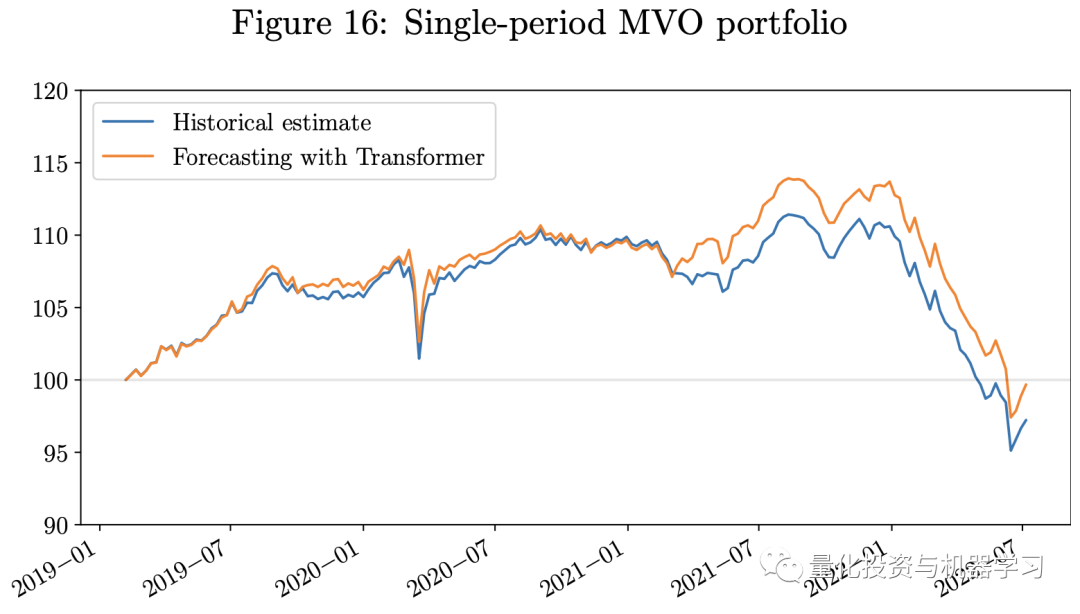
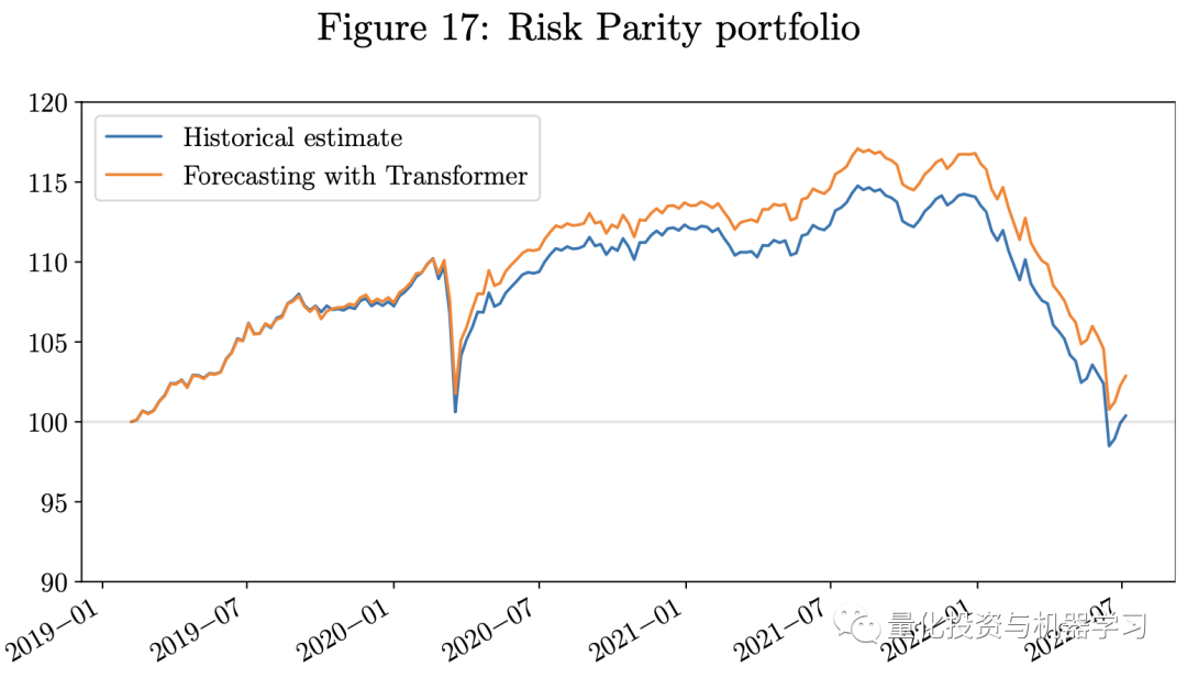
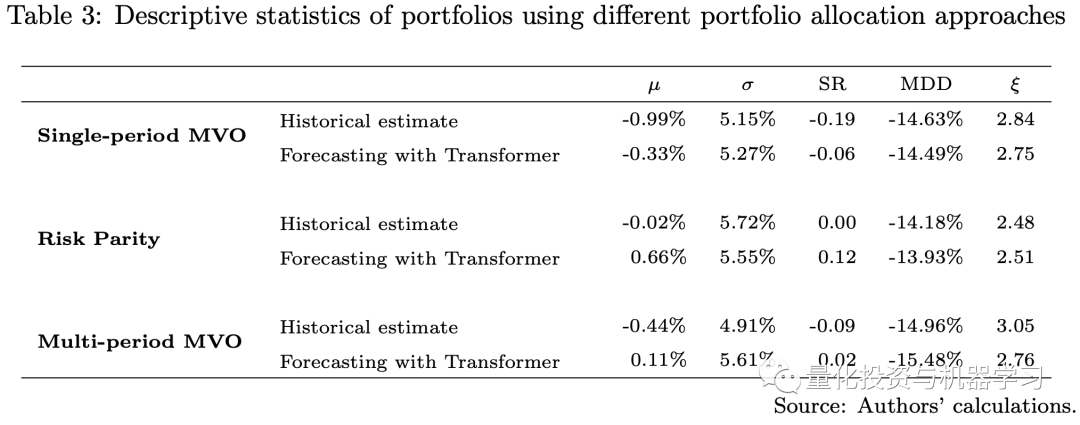
In our experiment, we consider three different portfolio allocation methods:
1. Monthly rebalancing based on MVO
2. Monthly rebalancing based on risk parity
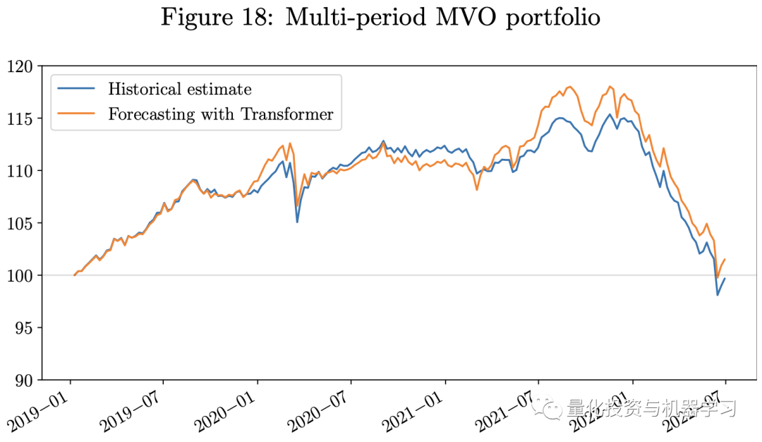
3. Weekly rebalancing based on multi-period MVO
The following diagram shows the backtesting results. Given that our testing period coincided with the economic challenges caused by COVID-19 and the Russia-Ukraine war, all three portfolios are long-only portfolios that experienced significant losses in 2022.However, the portfolio using predictions from the Transformer model outperformed those using historical estimates. The portfolio using the Transformer model had a higher Sharpe ratio. Our weekly rebalancing multi-period MVO portfolio outperformed the single-period MVO portfolio. Since the risk parity portfolio uses only the estimates of the VCV matrix as input, we do not include the estimation errors of returns in the model, which are often more challenging to estimate than the VCV matrix. Therefore, during this economically challenging period, the risk parity portfolio performed better than the MVO portfolio.
 As we described in this article, one of the main difficulties in applying machine learning techniques in finance is that the signal-to-noise ratio in financial data is often weak. Therefore, the next stage of research will focus on denoising and labeling financial data, which is key to the successful application of machine learning techniques in finance. Feature engineering is also important for time series forecasting, and we can decompose time series into trend, seasonal, and noise components using pattern decomposition techniques. Combining these methods with deep learning models is an interesting research topic. Secondly, as we described in the working paper on graph neural networks (Pacreau et al., 2021), attention mechanisms are also used in Graph Attention Layers (GAT) to capture underlying relationships between dimensions of data. Therefore, attempting to combine Transformer models with Graph Neural Networks (GNNs) to manage multivariate, spatiotemporal time series data, such as traffic forecasting, is very effective. Some researchers claim that this combination of models can improve performance and better understand causal relationships in spatiotemporal time series forecasting, as noted by Cai et al. (2020) and Xu et al. (2020).
In finance, the interrelationships between multiple companies or supply chain relationships can be viewed as spatial relationships. Therefore, combining Transformers and GNNs to model the dynamics and dependencies between time series and dimensions is an important avenue for our future research. This will open the door to a new research field to capture more complex relationships in financial data and improve quantitative investment strategies.
Cai, L., Janowicz, K., Mai, G., Yan, B., and Zhu, R. (2020), Traffic Transformer: Capturing the Continuity and Periodicity of Time Series for Traffic Forecasting, Transactions in GIS, 24(3), pp. 736-755.
Vapnik, V. (2000), The Structure of Statistical Learning Theory, Second edition, Springer.
Vaswani, A., Shazeer, N., Parmar, N., Uszkoreit, J., Jones, L., Gomez, A.N., Kaiser, L., and Polosukhin, I. (2017), Attention is all you need, NIPS’17: Proceedings of the 31st International Conference on Neural Information Processing Systems.
Pacreau, G., Lezmi, E., and Xu, J. (2021), Graph Neural Networks for Asset Management, ResearchGate, https://www.researchgate.net/publication/356634779.
As we described in this article, one of the main difficulties in applying machine learning techniques in finance is that the signal-to-noise ratio in financial data is often weak. Therefore, the next stage of research will focus on denoising and labeling financial data, which is key to the successful application of machine learning techniques in finance. Feature engineering is also important for time series forecasting, and we can decompose time series into trend, seasonal, and noise components using pattern decomposition techniques. Combining these methods with deep learning models is an interesting research topic. Secondly, as we described in the working paper on graph neural networks (Pacreau et al., 2021), attention mechanisms are also used in Graph Attention Layers (GAT) to capture underlying relationships between dimensions of data. Therefore, attempting to combine Transformer models with Graph Neural Networks (GNNs) to manage multivariate, spatiotemporal time series data, such as traffic forecasting, is very effective. Some researchers claim that this combination of models can improve performance and better understand causal relationships in spatiotemporal time series forecasting, as noted by Cai et al. (2020) and Xu et al. (2020).
In finance, the interrelationships between multiple companies or supply chain relationships can be viewed as spatial relationships. Therefore, combining Transformers and GNNs to model the dynamics and dependencies between time series and dimensions is an important avenue for our future research. This will open the door to a new research field to capture more complex relationships in financial data and improve quantitative investment strategies.
Cai, L., Janowicz, K., Mai, G., Yan, B., and Zhu, R. (2020), Traffic Transformer: Capturing the Continuity and Periodicity of Time Series for Traffic Forecasting, Transactions in GIS, 24(3), pp. 736-755.
Vapnik, V. (2000), The Structure of Statistical Learning Theory, Second edition, Springer.
Vaswani, A., Shazeer, N., Parmar, N., Uszkoreit, J., Jones, L., Gomez, A.N., Kaiser, L., and Polosukhin, I. (2017), Attention is all you need, NIPS’17: Proceedings of the 31st International Conference on Neural Information Processing Systems.
Pacreau, G., Lezmi, E., and Xu, J. (2021), Graph Neural Networks for Asset Management, ResearchGate, https://www.researchgate.net/publication/356634779.