On March 28, the 16th lecture of the “New Youth in Autonomous Driving” organized by Zhixingshi successfully concluded. In this lecture, Yang Zhigang, the core developer of the Horizon toolchain, conducted a live explanation on the topic of “Practical Experience in Transformer Quantization Deployment Based on Journey 5 Chip.”
Yang Zhigang first introduced the development trends of Transformers and the challenges of deploying them on embedded intelligent chips. He then focused on the algorithm development process for embedded intelligent chips using Journey 5 as an example, and provided a detailed interpretation of the quantization accuracy improvement and deployment performance optimization using SwinT as an example. Finally, he analyzed how to deploy the Transformer model efficiently and effectively on Journey 5.
This lecture was divided into two parts: the main lecture and Q&A. Click Read the Original to watch the complete live replay. The following is a review of the main lecture:
Hello everyone, my name is Yang Zhigang, and I am mainly responsible for the development of the Tiangong Kaiwu toolchain at Horizon, such as the development and verification of a series of quantization tools and algorithm tools on Journey 2, Journey 3, and Journey 5. Therefore, I have had in-depth contact with our company’s internal algorithm team and compiler team.
Today, the topic I will share is “Practical Experience in Transformer Quantization Deployment Based on Journey 5 Chip,” and I will analyze how to make Swin-Transformer run efficiently and effectively on Journey 5 from the aspects of quantization and deployment.
The main content of this lecture is roughly divided into four parts:
1. Development trends of Transformers and the challenges of deploying them on embedded intelligent chips
2. Algorithm development process for embedded intelligent chips using Journey 5 as an example
3. Quantization accuracy improvement and deployment performance optimization using SwinT as an example
4. How to deploy Transformer models efficiently and effectively on Journey 5
Development Trends of Transformers
and the Challenges of Deploying on Embedded Intelligent Chips
The first part discusses the development trends of Transformers and the challenges of deploying them on embedded intelligent chips. Recently, I believe everyone is aware of the unstoppable trend of Transformers, which indeed has played an irreplaceable role in the fields of NLP and even image processing. For example, since the introduction of Transformers in 2017, due to their powerful sequence modeling and global modeling capabilities, the Transformer model structure has increasingly occupied an important position in the entire intelligent model structure.
On one hand, it has led a trend towards large models (this trend mainly refers to the NLP field), such as the recent popular BERT, GPT, and other models based on Transformers, which have brought fundamental changes in the NLP field. The parameter count of models like GPT has increased from hundreds of millions to hundreds of billions, indicating that the capacity of Transformers and the trend of model development are moving towards larger scales. Of course, the premise for larger models is that we can achieve higher accuracy with them, so the scale has essentially moved from hundreds of millions to hundreds of billions and trillions.
On the other hand, Transformers are not only leading the trend of large models in the NLP field but also have increasingly important positions in the image field. The chart I have taken (as shown in Figure 1) mainly illustrates its trend in Backbone, specifically for classifying ImageNet. We can see that as its computational and parameter counts increase, its accuracy also improves. In fact, in common foundational tasks (such as detection, segmentation, tracking, etc.), when making leaderboard submissions, we can see that the top spots are almost all occupied by Transformers. Therefore, common models like Swin-Transformer as encoders and DETR as decoders, along with temporal and BEV models that use Transformers for feature fusion, have become common practices in various stages of the image field. Overall, Transformers have become an indispensable model structure in the current image domain.
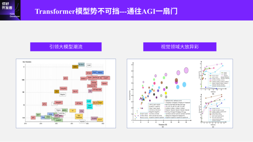
In fact, I added a phrase in the title: “A Door to General Artificial Intelligence.” Of course, I do not dare to claim this; I have seen it in some other information. It is now widely believed that during the feature extraction phase, Transformers are a component of general artificial intelligence, hence referred to as a door, but this is not the focus of our discussion today.
Transformers indeed play an increasingly important role in model structure, but on the other hand, the challenges of deploying them on embedded platforms are receiving more attention. Specifically, the increasing size of Transformers and the deployment on embedded intelligent chips are fundamentally different. For example, while Transformer models are becoming larger and wider, embedded intelligent chips are constrained by cost, power consumption, and other factors, leading to limitations in many functions such as computing power and bandwidth. This results in current embedded intelligent chips struggling to deploy even slightly larger or smaller Transformer models.
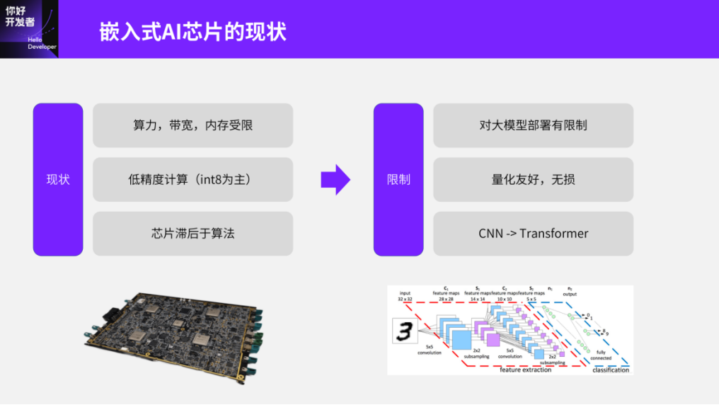
Figure 2
Here, I will discuss three main examples. The first is that embedded intelligent chips are limited by cost and power consumption, leading to restrictions on their computing power, bandwidth, and memory. This directly causes the deployment of large models like Transformers to be constrained. If we deploy a large model on a low-power platform, even if it is not a Transformer, but just a regular CNN, the performance will obviously be poor, let alone deploying a large model like a Transformer on a low-power platform, which will clearly have defects.
The second characteristic is that the currently popular embedded intelligent chips generally process deployed models in a low-precision manner. Of course, besides low precision, they also support a small amount of certain precision floating point operations. This is primarily due to considerations of cost and power consumption, which directly leads to the necessity of quantizing the model for deployment on embedded intelligent chips, while ensuring that quantization does not incur significant accuracy loss. Otherwise, if the accuracy loss is substantial, the deployment becomes meaningless.
The third point is that the development of chips actually lags behind algorithms. Regarding this, there is a detailed description in a previous sharing by our company’s Dr. Luo (Horizon Dr. Luo Heng: How to Build a Good Autonomous Driving AI Chip), which you can check out if interested. In brief, the process from chip design to mass production can take a long time, typically 2-4 years. Therefore, the embedded intelligent chips currently on the market are mostly based on designs that are 1-2 years or even longer old, and at that time, the designs likely did not consider Transformers, as most popular models were still based on CNNs. This results in most embedded intelligent chips being very friendly to CNN deployments but having a gap in deploying Transformers. Today, we will discuss where this gap comes from.
Next, let’s break down the issues encountered during the deployment of Transformers.
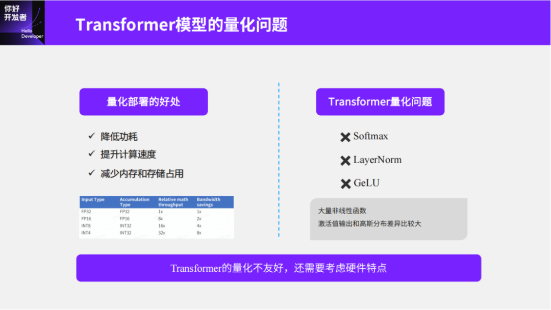
Figure 3
The first issue is quantization. In fact, we can see many papers or blogs in various communities discussing the quantization of Transformers. First, why does it need to go through quantization? As I briefly mentioned, this is due to considerations of cost and power consumption. The benefits of deploying using int8 or low-bit quantization are evident, such as reducing power consumption, increasing computation speed, and decreasing memory and storage usage. Here is a data comparison; there are some common issues when deploying Transformers. Those familiar with quantization training should be aware that there are many non-linear functions in Transformer models, such as GeLU and LayerNorm. Therefore, the output of activation values can have significant differences from Gaussian distributions, which directly leads to noticeable accuracy issues with the symmetric quantization methods that were commonly used in CNNs.
To address the quantization accuracy issues of Transformers, the community has shared many common experiences. For example, using asymmetric quantization methods to handle uneven distributions or significant differences from Gaussian distributions, and in some cases, directly using floating-point SoftMax or LayerNorm on the hardware can resolve quantization issues. However, we need to consider whether the hardware supports floating-point or asymmetric quantization. The Journey 5 platform we are discussing today is a pure int8 embedded intelligent platform, and deploying a floating-point SoftMax or LayerNorm on a pure int8 platform is clearly unreasonable. Even in some cases, even if it is pure int8, it may not support asymmetric quantization, so if we want to solve the issue of Transformers being unfriendly to quantization, we need to consider the characteristics of the hardware.
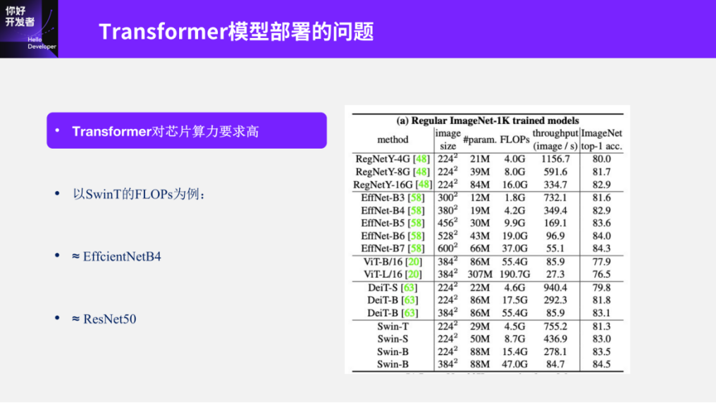
Figure 4
The second issue in deploying Transformer models is the high computational requirements. As mentioned earlier, Transformers are the most popular neural network model in recent years, and their most important and thorough application in machine vision is the Swin Transformer, which has also received the highest award in the machine vision field, the Marconi Prize. Here, we take the smallest model of Swin-Transformer as an example, which has a computational load of about 4.5G. Saying 4.5G might not give many people a clear idea, so I made two simple comparisons. This is roughly equivalent to the commonly used models like EffcientNetB4 and ResNet50. When it comes to ResNet50, many people might have a clearer understanding. If we deploy using the performance level of ResNet50, many slightly lower-powered embedded intelligent chips in the market would struggle to handle it. If someone knows the history of Horizon, they would know that the previous generation of Horizon chips could run ResNet50, but its efficiency was not very high, and this was still the deployment efficiency of CNNs. If we consider deploying Transformers, the efficiency would further decrease. Therefore, the precondition for deploying SwinT is that the chip’s computational power must meet certain requirements.
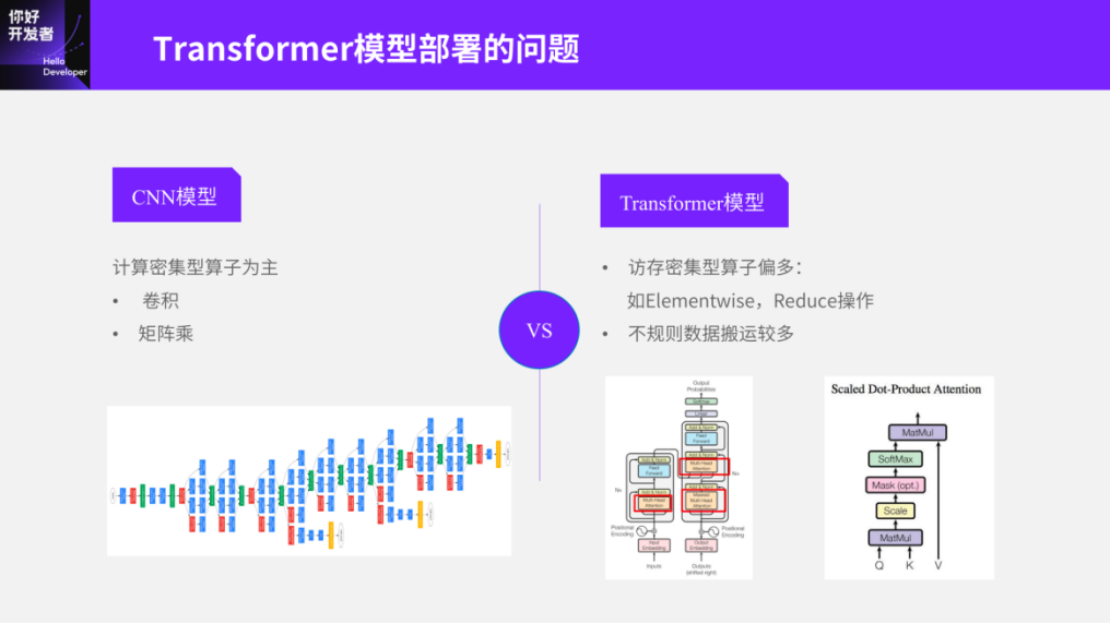
Figure 5
In addition to the quantization issue mentioned earlier and the foundational requirements of SwinT, there is another significant issue: the differences between Transformer and CNN models. Why is it that my chip can deploy ResNet50, but not Transformers? This is actually a crucial distinction between CNN and Transformer models. If we are familiar with CNN models, we know that CNNs primarily consist of convolutions, or a few non-convolutional operators, such as RoiAlign. In other words, the characteristics of this type of operator are mainly computation-intensive operators. The reason our early intelligent chips had strong concurrency ability is that they were designed with CNN models in mind, focusing on using concurrency to solve computation-intensive problems.
However, in Transformers, the situation is different. In addition to convolutions and matrix multiplications, there are many memory-intensive operators like Elementwise and Reduce. Memory-intensive operators and computation-intensive operators have obvious differences, requiring higher memory bandwidth or storage capacity, along with more irregular data movement. Unlike CNNs, where a 4d-tensor can be processed from start to finish with very clear rules: the W/H dimensions perform downsampling, and the C dimension varies in features, making this 4d-tensor characteristic very friendly to the entire embedded intelligent platform. But in Transformers, irregular data movement is much more prevalent. For example, in Swin-Transformer, during window partitioning and reversing, many Reshape and Transpose operations occur. This brings about efficiency issues, and in fact, this problem is encountered across the entire Transformer or chip industry, not just with embedded intelligent chips, but also with training chips.
I recall that a few years ago, NVIDIA conducted a simple OPS statistics test, which I won’t go into detail about, but the general conclusion is that purely computation-oriented operators like convolutions and matrix multiplications account for about 99.8% of the computational load, yet their execution time on NVIDIA chips (specifically for training chips) only accounts for 60%. In other words, training chips have a large proportion of low-occupancy non-computation operators, but these operators consume 40% of the time. This issue becomes significantly magnified when deploying Transformers on embedded intelligent chips. Common embedded intelligent chips may waste a lot of time on memory operators and irregular data movements.
To summarize the first part, embedded intelligent chips face significant differences in design philosophy and the actual Transformers that need to be deployed due to constraints like cost and power consumption.
Algorithm Development Process for Embedded Intelligent Chips Using Journey 5 as an Example
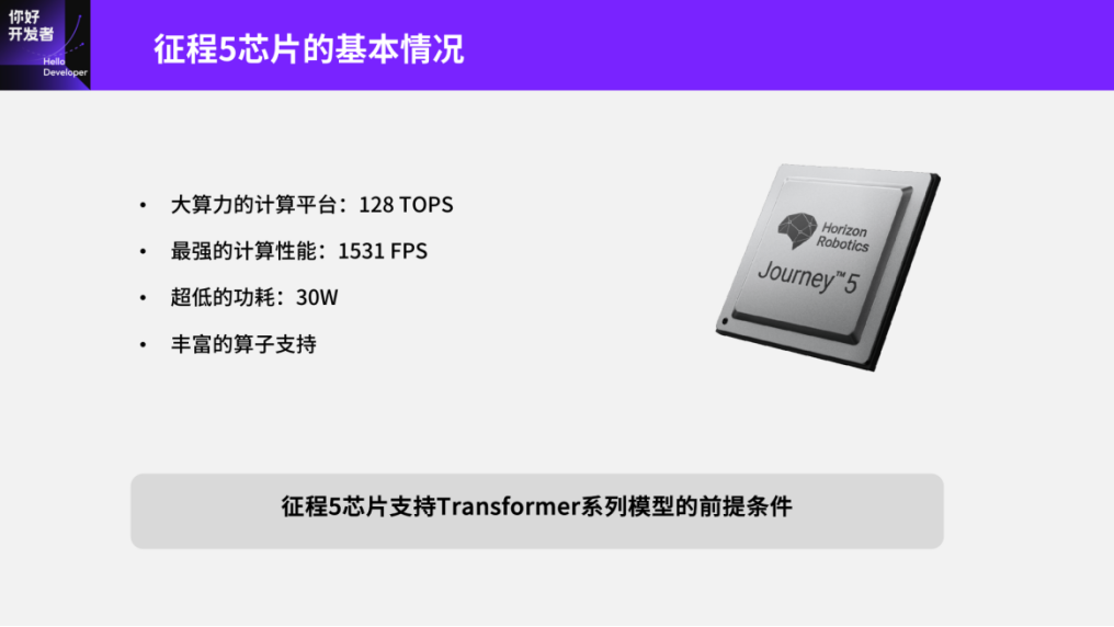
Figure 6
The second part focuses on the development process of embedded intelligent chips. Although this is based on Journey 5, our current research indicates that the development processes of most embedded intelligent chips are generally consistent, meaning that the issues everyone needs to solve are quite similar.
First, let’s briefly discuss the basics of Journey 5, which has been thoroughly described in previous series of lectures, detailing how Journey 5 was designed and what innovations or uses it has for intelligent driving platforms. I won’t elaborate too much here; I will mainly discuss how these basic conditions align with the prerequisites for deploying Transformers, which corresponds to the common deployment flaws of embedded intelligent chips.
The first point is the need for a high-performance computing platform. We must have a high-performance computing platform as a prerequisite to deploy Transformer series models. If the computing power is low, as mentioned earlier, deploying Transformers on the previous generation, Journey 3, could be quite challenging.
The second key point is rich operator support. As we saw in the structural diagram of Transformers, the main body of CNN models is based on convolutions with a few additional operators, such as RoiAlign. However, Transformers involve many diverse operators, such as LayerNorm, SoftMax, Reshape, and Transpose. Hence, the deployment of Swin-Transformer or other Transformers on intelligent chips requires not only high performance but also a comprehensive understanding of a wide variety of operators.
Additionally, the strongest computational performance is not particularly relevant for deploying Transformers, as it is based on CNN models, which are computation-intensive. However, the capabilities of Transformers exhibit a significant gap compared to this.
The last point is ultra-low power consumption, which also needs more discussion as it is one of the highlights of Journey 5. The Journey 5 chip and the Tiangong Kaiwu toolchain have accumulated a relatively complete set of software tools, starting from user training of floating-point models, followed by quantization, training, compilation, and optimization, ultimately deploying to the embedded side. For example, in terms of quantization, the entire chip toolchain provides both post-training quantization (PTQ) and quantization-aware training (QAT) methods. During the optimization compilation phase, tools such as Checker, Calibrator, and analysis/simulation are available to ensure that users’ models can be deployed on the embedded side after quantization and optimization. It is worth mentioning that the early Tiangong Kaiwu toolchain was built primarily on CNN models, and I will explain later why the entire chip toolchain, which was developed based on CNN models, has certain shortcomings when processing Transformer models, both in terms of quantization and optimization deployment.
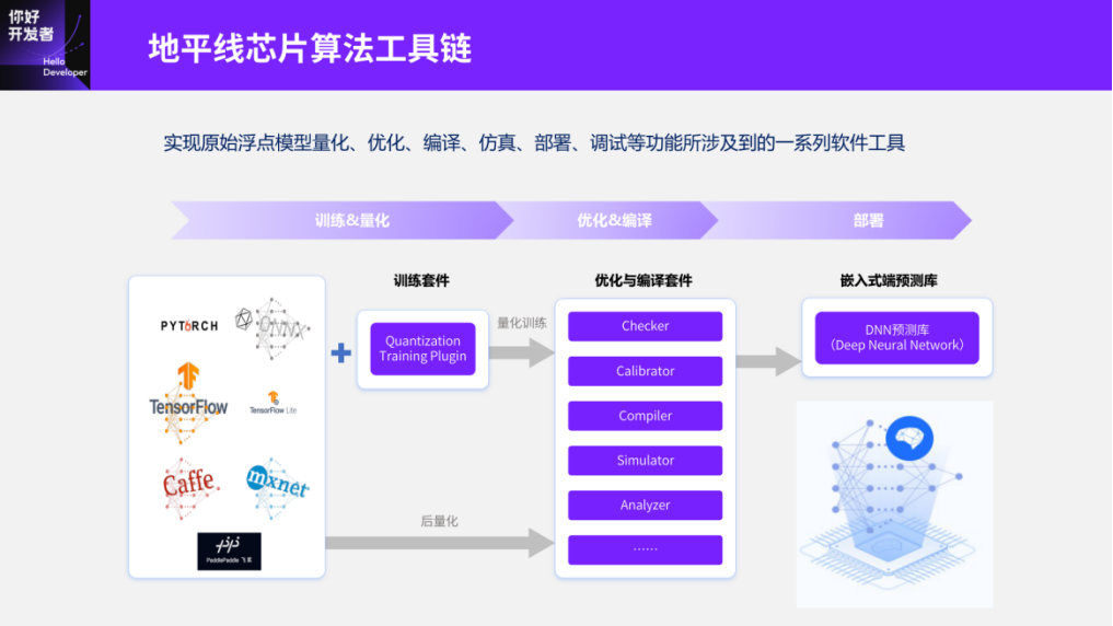
Figure 7
Next, let’s look at how to use the entire Tiangong Kaiwu toolchain to help users quickly deploy floating-point models to embedded chips. As I mentioned earlier, the deployment processes of different chip toolchains and embedded intelligent chips have become increasingly similar, generally considering the cost of algorithm migration, so it has essentially become a standardized process. Now, let’s examine this process: starting from floating-point training, followed by calibration for post-quantization, if the post-quantization accuracy meets the requirements, we can directly compile and optimize for deployment; if not, we can revert to perform quantization-aware training to achieve the required accuracy and ultimately define the model. If we want to optimize deployment for Transformers, the two key areas to address are quantization tuning and compilation optimization, mainly using quantization formulas to enhance quantization accuracy and improving deployment performance through manual or automated methods during the compilation process.
Tiangong Kaiwu toolchain successfully deployed Swin-Transformer on Journey 5 without encountering many difficulties. Of course, the prerequisites I mentioned earlier were essential: high performance and rich operator knowledge. These two aspects made the deployment process on Journey 5 relatively straightforward. Let’s briefly discuss which operators are supported. Those familiar with Swin-Transformer should understand that it includes operators like Reshape, roll, LayerNorm, matmul, etc. Why is complete operator support necessary? When we initially carried out this task, we found that ONNX opset did not fully support roll, so we had to handle the roll situation separately when testing Swin-Transformer on other brands. Recently, we discovered that the opset now supports roll, but this indicates that some embedded intelligent chip platforms face certain thresholds in achieving complete operator support, whether due to the tools used or the limitations of the final deployed chips.
The second point is quantization accuracy. Overall, after QAT, the quantization accuracy lost about 4 points. It should be noted that while a loss of 4 points may not seem disastrous, we have already accumulated a series of precision debugging tools and enhancement methods in our previous toolchain. However, its limitations may stem from being primarily based on CNN models, where we can usually quickly pinpoint where the quantization loss originates. When mapping some experiences onto Transformers, it is not as universally applicable. Therefore, based on the accumulation of experiences with CNNs, we achieved a loss of 4 points.
The final concern is the initial deployment FPS being less than 1, which indicates extremely low performance, essentially rendering it unusable. For reference, other CNN models on Journey 5, such as ResNet50, can exceed 600 FPS, while EffcientNet LiteB4 can exceed 1000 FPS. In reality, if it is a highly efficient model designed by Horizon, this number could be even higher. However, our concern is not the CNN issue but rather the unresolved gap between CNN and Transformer deployments, indicating that the bottlenecks in Transformer deployments cannot be directly addressed using CNN experiences.
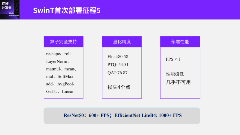
Figure 8
To summarize the second part, the standardized processes accumulated on Journey 5 through the Tiangong Kaiwu toolchain can effectively address CNN issues but cannot fully resolve the quantization deployment issues of Transformers. Therefore, I will now explain how to enhance quantization accuracy and optimize deployment performance using Swin-Transformer as an example.
Quantization Accuracy Improvement and Deployment Performance Optimization Using SwinT as an Example
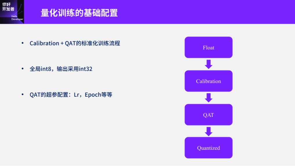
Figure 9
First, regarding the foundational configurations or standard processes accumulated with CNNs, what does this standard process entail? This requires discussing the basic configurations for quantization training in the Tiangong Kaiwu toolchain. However, there is no need to delve into PTQ post-quantization since besides some flexibility in method selection, there isn’t much room for training. Therefore, we will focus on the technical configurations for quantization training. In previous demonstrations, we separated PTQ from QAT, meaning either executing PTQ post-quantization or using QAT quantization training. However, we found through experience that using PTQ post-quantization parameters to initialize QAT can provide a higher starting point for QAT’s initial state, ensuring faster convergence during quantization training. Therefore, the current quantization training process, whether for CNNs or Transformers, essentially follows a PTQ + QAT workflow, which has become a standardized operation. Additionally, common configurations for CNNs include using int8 globally while using int32 only at the output stage. During the QAT process, some hyperparameter configurations such as learning rates typically set at 10^-3 or 10^-4, and epochs generally being 10%-20% of floating-point training, do not need extensive elaboration; those with quantization training experience will likely be familiar with these.
Next, let’s discuss how to fine-tune quantization accuracy. We strongly advise against blindly attempting more methods during PTQ or arbitrarily adjusting QAT parameters. Instead, we recommend using more reasonable methods that can quickly analyze the sources of quantization loss. For instance, we generally categorize quantization loss errors from a tool perspective into three parts: operator error, model error, and precision error. Many people are likely aware of how a single operator’s error behaves after quantization. Model error refers to situations where, under the same input conditions, we identify some FeatureMaps that are relatively large or have uneven distributions, which can be very unfriendly to quantization. This may also include errors in model parameters, such as weights; if certain weights are notably large after training, this can also adversely affect quantization. Finally, precision error typically involves using distributed quantization methods to determine which module in the model contributes most to the overall dataset and model error.
The following two images provide visual results from our quantization loss analysis tool, allowing us to intuitively see the errors originating from operators or the model itself, as well as weight distribution errors. The second issue is how to address large computation errors once identified. A simple approach is to use floating-point operations as mentioned earlier, but if the chip does not support floating-point operations, we should seek other higher precision representations. For instance, Journey 5 supports a small number of int16 operations, but int16 may not be natively supported; we can piece together int16 from int8 operations. Therefore, if we want to express certain operators with higher precision, we should prioritize using int16.
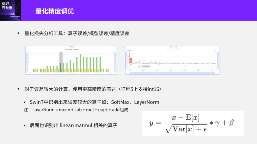
Figure 10
On the other hand, if we want to deploy Transformers more effectively on the next generation of chips or embedded intelligent chips that are friendly to Transformers, some operators may yield better results using floating-point methods. Here, we primarily use int16 methods to address quantization errors. For example, in the quantization process for LayerNorm, we actually decompose LayerNorm into specific operators like addition, subtraction, multiplication, division, and square root, and all intermediate results, except for input and output, such as means and additions, are performed using int16 methods. This approach allows LayerNorm or SoftMax—two operators that tend to have larger errors—to achieve higher precision representations. Many may argue that SoftMax and LayerNorm do not require such measures to identify quantization loss errors, as I initially mentioned, their output distribution range clearly does not conform to Gaussian distributions, or as seen with GeLU. However, in subsequent detection experiments, we found that certain special linear or matmul operations can yield better precision results when specifically using int16, such as using int16 for linear inputs or int16 for certain matmul outputs.
The second part addresses the issues of compilation and deployment optimization after resolving quantization accuracy. Here, I will present some basic statistical data, which reflects the initial deployment situation of the compiler or Swin-Transformer on Journey 5. The first is that the ratio of tensor (Tensor) to vector (Vector) calculations is approximately 218:1. Tensor calculations refer to matrix multiplications, convolutions, etc., while vector calculations pertain to normalization operations. The calculation ratio here is about 218:1. This number may not be apparent at first glance, but we can compare it with CNNs; if the vast majority of models yield tensor calculation results, this ratio can approach infinity. In such cases, embedded intelligent computing platforms designed for concurrency can better exploit their parallel efficiency. However, this ratio indicates that the chip itself will require more time to handle vector calculations. Additionally, the high proportion of Reshape and Transpose data movement operators may also relate to historical issues, as CNNs did not encounter these types of operators in practical applications, leading to suboptimal functionality and performance optimizations, which is one of the reasons for the extremely low deployment efficiency of Swin-Transformer.
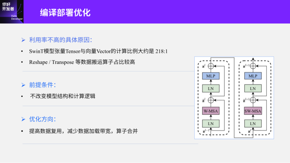
Figure 11
Now, let’s discuss our overall optimization for the compiler deployment, with the premise being that we should not alter the overall model structure and computation logic. Regardless of how we optimize, users should not need to retrain floating-point or quantized models. If we can lower this cost, users can simply perform equivalent replacements as needed. The optimization direction involves common compiler optimization strategies, such as improving data reuse, reducing data loading bandwidth, and merging operators.
Next, let’s highlight specific operations. We have summarized five optimization directions, some of which require algorithm-side awareness, while others can be accomplished directly by the compiler without requiring algorithm awareness. We will mention these in the explanation.
The first is operator mapping optimization. In simple terms, this involves enhancing the functionality of operator implementations on the compiler side, allowing each computational unit or component to cover more functionalities. This way, individual operators can perform multiple functions, thereby increasing parallel opportunities within the operator. For instance, in QAT self-attention, we generally use matmul, and Transpose is often paired with matmul. From the compiler’s perspective, matmul can incorporate Transpose, thereby enabling a single matmul operator to complete both functions while enhancing parallel opportunities.
Similarly, in the case of LayerNorm, if there are view or Transpose operations before and after, we can merge the dimensional changes into the upper layer. This allows us to use a custom operator to support a rich variety of dimensions, enabling view operations to achieve effects similar to those of Transpose. However, this interface modification requires user awareness; it is only available through the operator interfaces provided in the Tiangong Kaiwu toolchain. Of course, this is purely for performance optimization, and using the original interface for support or deployment remains unobstructed.
The second part is operator fusion. Operator fusion is relatively straightforward; the data layout of Journey 5 is a multidimensional representation, while Reshape and Transpose operations describe the numerical behavior of CPU and GPU. Therefore, if I want to perform multiple, consecutive, linear rearrangements on Journey 5, theoretically, Journey 5 can achieve a unified layout in one go.
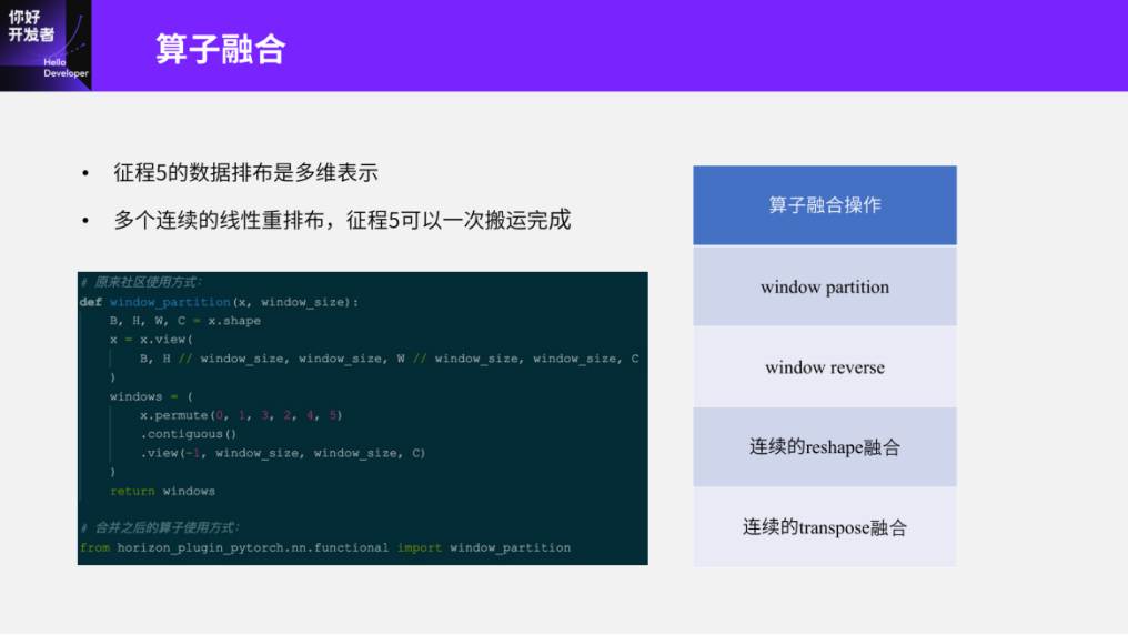
Figure 12
It is particularly evident with the window partition and window reverse operators, which mainly involve Reshape, view, and permute operations, essentially dealing with irregular data movements. For Journey 5, our optimization direction is to merge these into a single operator for execution, thus allowing us to define a custom window partition that doesn’t require awareness of detailed logic like view or permute. From the compiler’s perspective, a single instruction can accomplish the window partition operation. In other words, whether multiple operators can be fused together and whether this can be accomplished through graph optimization or automatically by the compiler without requiring algorithm-side awareness is theoretically possible. However, another issue with graph optimization is that it requires maintaining numerous patterns, meaning that only under these optimization rules can we achieve the final optimization effect. Let’s take a look at the dimensional information of window partitioning and various format changes; I can derive a plethora of writing styles from this. If we want to maintain all patterns during the subsequent compilation stage for automated graph optimization, it would be less efficient than using a fixed format with parameters for user use at the operator level, and this replacement incurs almost no cost and does not require retraining. Besides window partitioning and window reversal, there are also common graph optimizations like merging consecutive Reshape and Transpose operations, which can be achieved through automated graph optimization without requiring user awareness.
Another key aspect is operator implementation optimization. Although this may not seem very important, it can effectively enhance performance. As we mentioned, certain historical factors, such as the limited use of Reshape and Transpose in early CNN models, led to the use of DDR for implementing operators on Journey 5. To improve performance, we moved the DDR implementation to SRAM, resulting in significant performance enhancements for deploying Transformers. We will provide detailed data to illustrate this later.
Another feature is the optimization of Batch MatMul, which is performed using ordinary loop tiling. Additionally, there are various other minor graph optimization tasks, such as elementwise operators or concat/split operators. If it involves obtaining a specific dimension through Reshape and Transpose, and only requires this dimension on the GPU or CPU, the dimension information can penetrate into the operators that need to be computed. For example, if I need to concat along a certain dimension and obtain this dimension through Reshape, the Reshape operation can potentially be fused into the concat operation, completing it in one go.
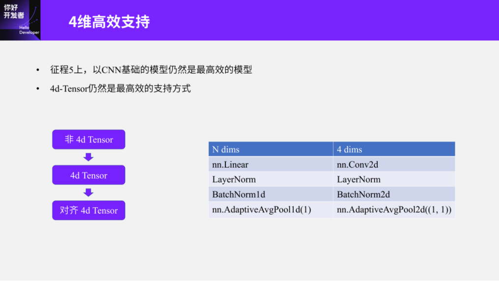
Figure 13
Furthermore, we have consistently stated that Journey 5 is very friendly to CNN models, but when it comes to Transformer models, apart from the graph optimizations mentioned above, there are still some evident gaps. The models based on CNNs are still the most efficient on Journey 5, which is reflected in the fact that regular 4d-Tensors remain the most efficient support method. Why emphasize regular 4d-Tensors? Because certain dimensional information in CNNs, such as W/H for downsampling and C for feature expansion, is very structured. Thus, on common embedded intelligent chip platforms, we usually have some basic alignment operations, and Journey 5 performs 4d-Tensor alignment. In simple terms, we can convert a non-4d-Tensor into a 4d-Tensor and align certain unimportant or determining dimensions, allowing the 4d-Tensor to combine with the common alignment operations of embedded intelligent chips. For instance, in Conv operations, I will elaborate on this later. Additionally, the channel dimension on Journey 5 is typically aligned to 8, and the W dimension to 16. If these two dimensions are converted from non-4d-Tensors to 4d-Tensors, considering their alignment, it may lead to complex alignments that significantly reduce computational efficiency and introduce many unnecessary calculations. Therefore, we generally recommend using a 4d computational logic where possible to replace operations on arbitrary dimensions, although this is not mandatory, as Journey 5 currently supports operations on arbitrary dimensions. If users aim to achieve higher performance manually, they can replace original operations with purpose-driven alignment of 4d-Tensor rules. For example, we could use nn.Conv2d to replace nn.Linear, which is an equivalent replacement. For instance, we can perform certain Reshape operations on weights and carry out dimensional fusion or expansions through Conv, which is also equivalent, and other operations like BatchNorm and LayerNorm should be considered in conjunction with Conv.
Finally, let’s conclude with the optimization of SwinT on Journey 5. Through the various optimizations mentioned earlier, we can reduce the quantization loss of Swin-Transformer to around 1%, while achieving a deployment efficiency of 143 FPS. We can look at the optimization options here; the optimization of Reshape and Transpose is particularly significant, and of course, other optimizations are also crucial. Compared to the initial FPS of less than 1, the improvements with Reshape and Transpose represent just the first step. It should be noted that the 143 FPS figure may differ from the 133 mentioned in previous documents published on WeChat, but we will consider 143 as the primary figure. After exploring various Transformer models, we found that this number has seen some enhancement in recent versions, potentially exceeding the previous figure by 10 FPS. Additionally, we compared this number with the strongest edge-side GPUs, finding that it is not significantly inferior. However, our power consumption is only about 50% of that of the strongest edge-side GPU, which is still quite impressive.
How to Efficiently and Effectively Deploy Transformer Models on Journey 5
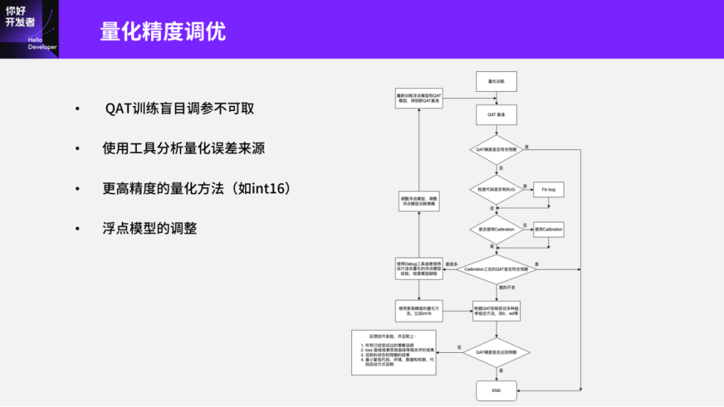
Figure 14
Finally, let’s discuss how to efficiently and effectively deploy Transformer models on Journey 5 while promoting the experiences of Swin-Transformer to all other Transformer models.
The first part is about tuning quantization accuracy. In fact, we have already discussed some aspects, such as our strong recommendation against blindly using PTQ methods and instead advising the use of quantization and analysis tools to analyze the sources of errors. Additionally, we do not recommend adjusting QAT parameters arbitrarily, as we can analyze the sources of errors from the tools, including operator errors, model errors, and precision errors.
We later discovered that model errors in Swin-Transformer can be quite challenging to analyze. Here’s a simple example regarding formats: in CNN models, Conv + BN is a standard format. The quantization of Conv + BN typically inserts quantization nodes before Conv and after BN, meaning that if the output range of Conv is large, it may not need quantization. The overall normalization after BN can facilitate quantization, so this part does not need consideration. However, in Transformers, we encounter a peculiar phenomenon: the output distribution of Linear is very large, while the subsequent normalization method is LayerNorm, which cannot be quantized together with Linear. Therefore, we observe a strange situation where similarity error analysis shows that the similarity error before Linear may not be high, yet it sharply increases after Linear, only to drop again after LayerNorm. This situation necessitates distinguishing whether the conclusions drawn from CNN regarding quantization nodes or model errors are very effective for Transformers. Moreover, we recommend using distributed quantization methods to analyze errors across the entire dataset or precision, which may be more reasonable. When encountering significant quantization errors, we suggest using higher precision quantization methods. This is not only more convenient on Journey 5 with int16 but also reasonable for other platforms using floating-point or FP16/BF16 operations.
The second aspect pertains to deployment recommendations. We strongly suggest using pre-packaged operators, such as window reverse, window partition, matmul, LayerNorm, etc. These can be accessed through the QAT or PTQ tools in the Tiangong Kaiwu toolchain. If interested, you can try using them later. Another commonly used operator available in the Tiangong Kaiwu toolchain, but not utilized in Swin-Transformer, is the MultiHeadAttention operator. Currently, the quantization tools themselves support operators and their deployment optimization.
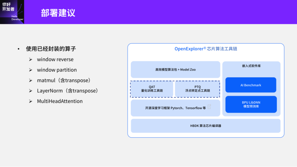
Figure 15
The third aspect is the alignment of tensors. I just briefly mentioned this in the deployment optimization of Swin-Transformer. Here, we outline the basic situation of Journey 5, including the basic operational components of Conv and the alignment strategies it supports. If we want to enhance the utilization of Journey 5 through detailed optimization, we can further boost deployment efficiency by combining 4d-tensor optimization ideas with patterns. Generally, Conv operations have H/W dimensions aligned to 26 or channel dimensions aligned to 8. If you are interested in alignment strategies, feel free to look directly.
Another point to mention is that in addition to the internal alignment waste of operators within single computational components, there are also some Reorder operator costs associated with switching between different components. The principle behind this cost is relatively simple: if the determining value of the previous computational component is small, for example, if the Conv’s channel dimension is determined to be 8, while the subsequent ReduceSum operator requires a channel dimension of 256, when we fit a Conv operator with a minimal determining value of 8 into ReduceSum, we end up performing a considerable amount of ineffective computations. This analysis serves as a rather unique example. A recommended method is to connect a Conv operator directly with a ReduceSum, ensuring that there is a relatively large determining value in the channel dimension. This way, when switching between Conv and ReduceSum, we can observe a notable Reorder overhead. One solution is to replace ReduceSum with convolution, which simplifies the computation method and is similar to our earlier Conv replacing linear operations. For example, if we perform reduction in the C dimension, the kernel size can be represented as (C, 1, 1, 1), effectively reducing the C dimension from its original value to 1, while reducing over H can be represented as (C, C, H, 1).
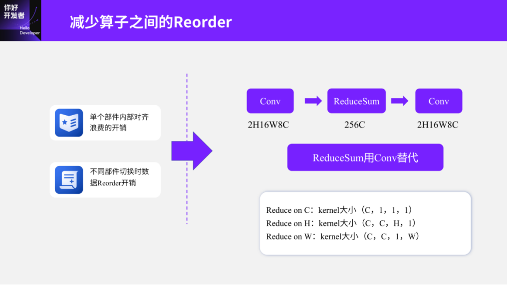
Figure 16
Finally, I would like to share some future work. Deploying SwinT on Journey 5 was part of our efforts last year. With the release of toolchain reference models, we will be publishing more Transformer models, such as DETR, DETR3d, PETR, etc. We will also be introducing more Transformer-related operators, quantization debugging tools, and experiences into the toolchain. Furthermore, we will explore more possibilities for deploying Transformer models in production on Journey 5. In fact, Swin-Transformer primarily served as a validation process to verify the feasibility of Journey 5. However, for production models with extremely high FPS requirements, we recommend embedding certain Transformer operations within CNN operations. For instance, we can refer to the current trend of optimizing MobileNet and ViT, or employ Transformer methods for feature fusion in BEV and temporal contexts, rather than relying on traditional convolution methods. This limited use of Transformers can not only enhance model performance but also improve deployment efficiency on Journey 5. Finally, we are already working on deploying Transformers in non-CV tasks, such as in speech processing.
Overall, that concludes my presentation. If anyone is interested, you can visit Horizon’s developer community (https://developer.horizon.ai/), where you will find more details about the toolchain, open documentation, and reference algorithms. If you have any questions, feel free to engage in discussions there.
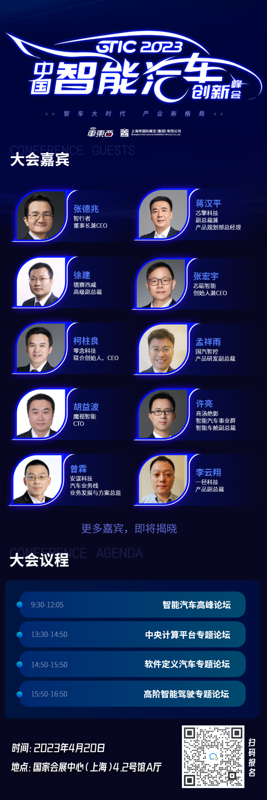
On April 20, the GTIC 2023 China Intelligent Vehicle Innovation Summit will be held concurrently with the Shanghai Auto Show. Confirmed speakers include Zhang Dezhiao, CEO of Zhixingzhe; Hu Yibo, CTO of Moshi Intelligent; and Xu Jian, Senior Vice President of Desay SV, among others. Welcome to scan the QR code to register~
Click “Looking” and Chat with Everyone
👇👇👇