Applications of Deep Learning in Marketing

### 1. Article Basic Information

– **Article Title**: Deep Learning in Marketing: A Review and Research Agenda

– **Author**: Xiao Liu, New York University

– **Publication Location**: Chapter related to “Artificial Intelligence in Marketing Review of Marketing Research”

– **Main Idea of the Article**: To review the applications of deep learning (DL) in marketing, introduce the mechanisms of six popular algorithms, discuss the applicability of DL to marketing problems and the reasons for its growth in recent years, emphasize its ability to model unstructured data in the absence of formal theories and knowledge, and describe future research directions.

• Main Idea of the Article: To review the applications of deep learning (DL) in marketing, introduce the mechanisms of six popular algorithms, discuss the applicability of DL to marketing problems and the reasons for its growth in recent years, emphasize its ability to model unstructured data in the absence of formal theories and knowledge, and describe future research directions.

### 2. Background of DL Applications in Marketing

– **Characteristics of Marketing Data and Applicability of DL**

– The marketing process often involves large-scale and/or unstructured data, such as product design, promotional materials, etc. DL is good at processing unstructured data and can better manage the unstructured elements in marketing, thus expanding the scope of marketing research.

– **Development Process and Technical Basis of DL**

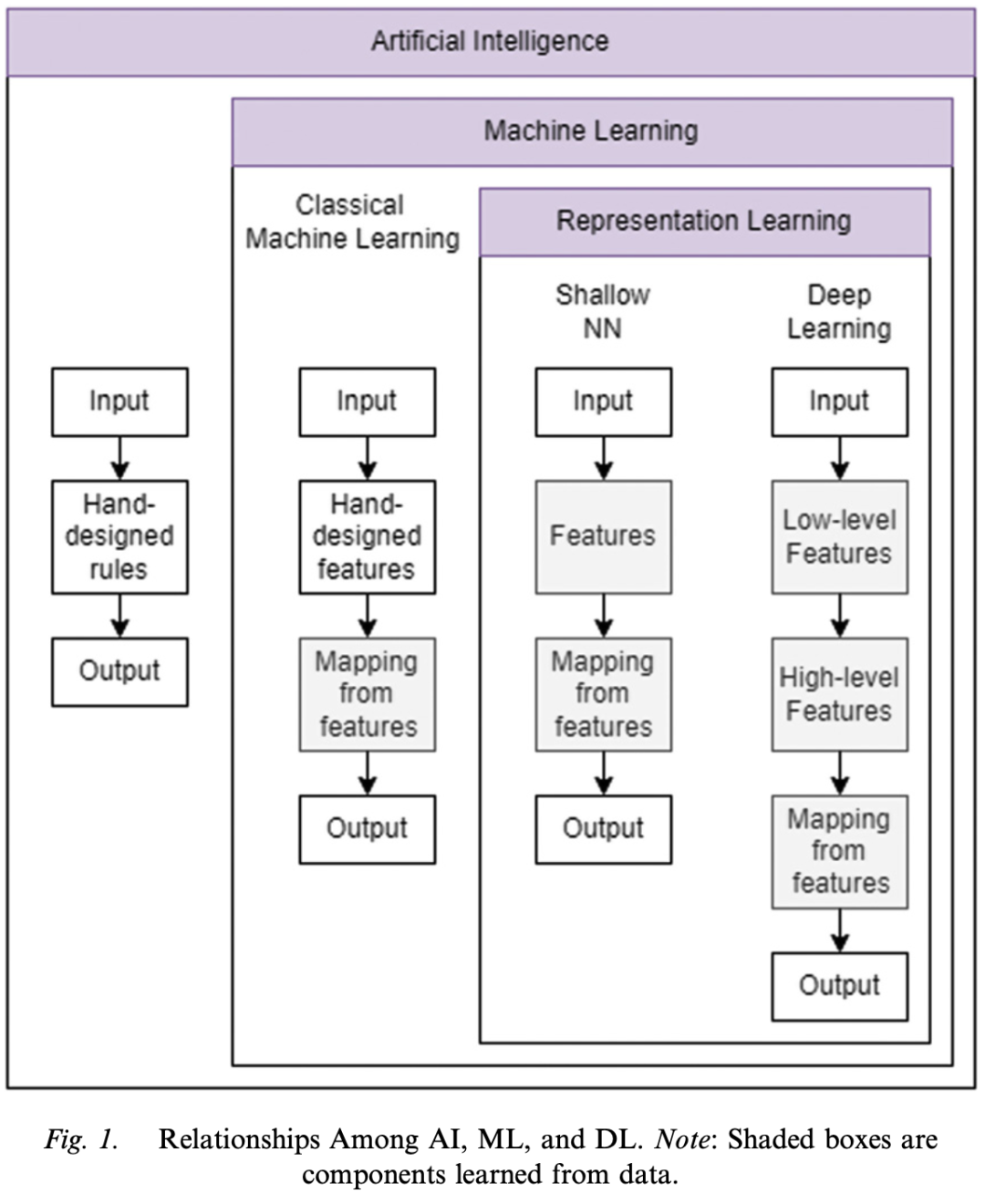
– DL is a special type of machine learning (ML) model and a subset of AI. In the early days of AI, rule-based systems were used. With the progress of research, ML (data-driven rather than rule-driven) emerged. However, classical ML requires manual feature design when processing unstructured data. DL further develops based on artificial neural networks (ANN) and can automatically learn hierarchical feature representations of data, overcoming the limitations of classical ML.

– **Reasons for the Growth of DL Applications in Marketing**

– Two factors have driven the growth of DL applications in marketing: one is the big data generated by the digitization of society, and the other is the performance breakthroughs of DL algorithms on many tasks to achieve human-level performance. Its high accuracy and efficiency enable marketers to use it.

• Characteristics of Marketing Data and Applicability of DL

• The marketing process often involves large-scale and/or unstructured data, such as product design and promotional materials. DL is good at processing unstructured data and can better manage the unstructured elements in marketing, thus expanding the scope of marketing research.

• Development Process and Technical Basis of DL

• DL is a special type of machine learning (ML) model and a subset of AI. In the early days of AI, rule-based systems were used. With the progress of research, ML (data-driven rather than rule-driven) emerged. However, classical ML requires manual feature design when processing unstructured data. DL further develops based on artificial neural networks (ANN) and can automatically learn hierarchical feature representations of data, overcoming the limitations of classical ML.

• Reasons for the Growth of DL Applications in Marketing

• Two factors have driven the growth of DL applications in marketing: one is the big data generated by the digitization of society, and the other is the performance breakthroughs of DL algorithms on many tasks to achieve human-level performance. Its high accuracy and efficiency enable marketers to use it.

### 3. Basics of Neural Networks

– **Basic Components of Neural Networks**

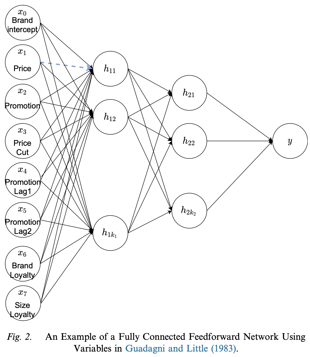
– The basic computational units of ANN are neurons, which are interconnected to form hidden layers and constitute the entire network. Taking the consumer discrete choice model as an example, it is introduced how a neural network predicts the output variable (consumer choice) through input variables (such as brand, price, etc.) and calculations in hidden layers.

• Basic Components of Neural Networks

• The basic computational units of ANN are neurons, which are interconnected to form hidden layers and constitute the entire network. Taking the consumer discrete choice model as an example, it is introduced how a neural network predicts the output variable (consumer choice) through input variables (such as brand, price, etc.) and calculations in hidden layers.

– **Main Components of Neural Networks**

– **Architecture**: The network architecture includes depth, breadth, adjacent layer connection type, and skip connections. It is a key part of designing a neural network and is usually regarded as a hyperparameter. Cross-validation and grid search are required to find the optimal settings.

– **Activation Functions**: The activation function used in each neuron is a design choice. Common ones include linear, logistic sigmoid, hyperbolic tangent, Softmax, and rectified linear units (ReLu).

– **Objective Function**: In ML, the cross-entropy loss function is commonly used as the objective function, which is essentially equivalent to maximum likelihood estimation (MLE). The goal is to minimize the distance (KL divergence) between the data distribution and the model distribution.

• Architecture: The network architecture includes elements such as depth, breadth, adjacent layer connection type, and skip connections. It is a key part of designing a neural network and is usually regarded as a hyperparameter. Cross-validation and grid search are required to find the optimal settings.

• Activation Functions: The activation function used in each neuron is a design choice. Common ones include linear, logistic sigmoid, hyperbolic tangent, Softmax, and rectified linear units (ReLu).

• Objective Function: In ML, the cross-entropy loss function is commonly used as the objective function, which is essentially equivalent to maximum likelihood estimation (MLE). The goal is to minimize the distance (KL divergence) between the data distribution and the model distribution.

– **Optimizers**: Given the objective function, an optimization method is required to find the model parameters. Common optimizers include gradient descent and second-order methods (such as BFGS). For DL, gradient descent and its variants (such as stochastic gradient descent, SGD) are more suitable because second-order methods have high computational costs.

– **Regularization (Dropout)**: DL involves many parameters and is prone to overfitting. The Dropout method prevents overfitting by randomly dropping a certain proportion of neurons. The dropout rate is a hyperparameter and can be adjusted by cross-validation.

• Optimizer: Given the objective function, an optimization method is required to find the model parameters. Common optimizers include gradient descent and second-order methods (such as BFGS). For DL, gradient descent and its variants (such as stochastic gradient descent, SGD) are more suitable because second-order methods have high computational costs.

• Regularization (Dropout): DL involves many parameters and is prone to overfitting. The Dropout method prevents overfitting by randomly dropping a certain proportion of neurons. The dropout rate is a hyperparameter and can be adjusted by cross-validation.

### 4. Deep Learning Algorithms

– **Discriminative Deep Learning Models** Discriminative Deep Learning Models

– **Convolutional Neural Networks (CNN)**

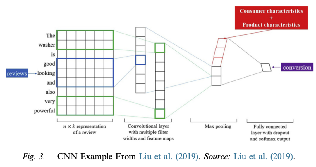
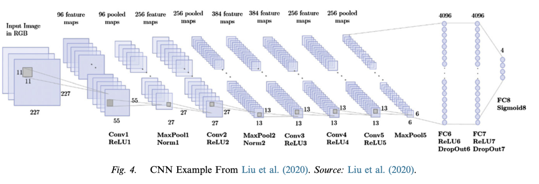
– **Model Mechanism**: CNN reduces the number of free parameters in a network through local sparse connectivity and parameter sharing and usually includes convolutional layers, pooling layers, and fully connected layers. Taking the impact of product review content on the sales conversion rate as an example, it is introduced how CNN processes text data by extracting local features and combining them to predict the result.

– **Advantages and Disadvantages**: The advantages are that it can provide an efficient dense network, is parallelizable, and can handle inputs of different sizes; the disadvantages are that it loses long-term dependencies when applied to sequence data.

– **Implementation Details**: It involves design choices such as window size and filter shape. Different data types may require different settings. CNN has been used to analyze text, image, and video data for marketing problems.

• Convolutional Neural Networks (CNN)

• Model Mechanism: CNN reduces the number of free parameters in a network through local sparse connectivity and parameter sharing and usually includes convolutional layers, pooling layers, and fully connected layers. Taking the impact of product review content on the sales conversion rate as an example, it is introduced how CNN processes text data by extracting local features and combining them to predict the result.

• Advantages and Disadvantages: The advantages are that it can provide an efficient dense network, is parallelizable, and can handle inputs of different sizes; the disadvantages are that it loses long-term dependencies when applied to sequence data.

• Implementation Details: It involves design choices such as window size and filter shape. Different data types may require different settings. CNN has been used to analyze text, image, and video data for marketing problems.

import tensorflow as tf
from tensorflow.keras import layers, models
# Define Convolutional Neural Network model
def create_cnn_model(input_shape):
    model = models.Sequential()
    # Add convolutional layers
    model.add(layers.Conv2D(32, (3, 3), activation='relu', input_shape=input_shape))
    model.add(layers.MaxPooling2D((2, 2)))
    model.add(layers.Conv2D(64, (3, 3), activation='relu'))
    model.add(layers.MaxPooling2D((2, 2)))
    model.add(layers.Conv2D(64, (3, 3), activation='relu'))
    # Add fully connected layers
    model.add(layers.Flatten())
    model.add(layers.Dense(64, activation='relu'))
    model.add(layers.Dense(10, activation='softmax'))
    return model
# Assume input shape is (64, 64, 3)
input_shape = (64, 64, 3)
model = create_cnn_model(input_shape)
# Compile model
model.compile(optimizer='adam',
              loss='sparse_categorical_crossentropy',
              metrics=['accuracy'])
# Print model summary
model.summary()

– **Recurrent Neural Networks (RNN)**

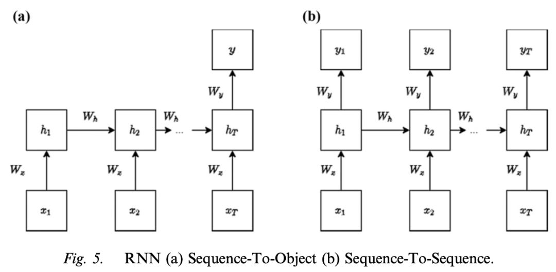
– **Model Mechanism**: RNN is suitable for processing input data with sequential information, such as words in a document or image frames in a video. In each time step, the hidden unit is updated by combining the current input and the previous hidden unit, and the final output is a function of the last hidden layer.

– **Advantages and Disadvantages**: The advantages are that it can incorporate historical information and the model size does not increase with the input data size; the disadvantages are that it is slow to compute and has a vanishing gradient problem for long sequences.

– **Implementation Details**: The basic RNN has no special hyperparameters to adjust. To solve the vanishing gradient problem, LSTM or GRU architectures can be used. RNN has been used for marketing applications dealing with text data.

• Recurrent Neural Networks (RNN)

• Model Mechanism: RNN is suitable for processing input data with sequential information, such as words in a document or image frames in a video. In each time step, the hidden unit is updated by combining the current input and the previous hidden unit, and the final output is a function of the last hidden layer.

• Advantages and Disadvantages: The advantages are that it can incorporate historical information and the model size does not increase with the input data size; the disadvantages are that it is slow to compute and has a vanishing gradient problem for long sequences.

• Implementation Details: The basic RNN has no special hyperparameters to adjust. To solve the vanishing gradient problem, LSTM or GRU architectures can be used. RNN has been used for marketing applications dealing with text data.

import tensorflow as tf
from tensorflow.keras import layers, models
# Define Recurrent Neural Network model
def create_rnn_model(input_shape):
    model = models.Sequential()
    # Add RNN layers
    model.add(layers.SimpleRNN(64, input_shape=input_shape, return_sequences=True))
    model.add(layers.SimpleRNN(64))
    # Add fully connected layers
    model.add(layers.Dense(10, activation='softmax'))
    return model
# Assume input shape is (100, 50)
input_shape = (100, 50)
model = create_rnn_model(input_shape)
# Compile model
model.compile(optimizer='adam',
              loss='sparse_categorical_crossentropy',
              metrics=['accuracy'])
# Print model summary
model.summary()

– **Transformer**

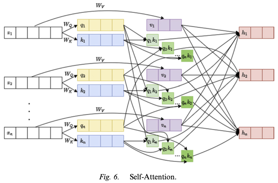
– **Model Mechanism**: Transformers are based on two key mechanisms: self-attention and position encoding. The self-attention mechanism allows input units to interact and determine weights, enabling parallelization and avoiding the vanishing gradient problem; position encoding inserts position information into the representation.

– **Advantages and Disadvantages**: The advantages are that it is faster than RNN and can better handle long sequences; the disadvantages are that it increases the number of weight parameters and training complexity.

– **Implementation Details**: Taking text classification as an example, the application of Transformers is introduced, involving the adjustment of multiple hyperparameters.

• Transformers

• Model Mechanism: Transformers are based on two key mechanisms: self-attention and position encoding. The self-attention mechanism allows input units to interact and determine weights, enabling parallelization and avoiding the vanishing gradient problem; position encoding inserts position information into the representation.

• Advantages and Disadvantages: The advantages are that it is faster than RNN and can better handle long sequences; the disadvantages are that it increases the number of weight parameters and training complexity.

• Implementation Details: Taking text classification as an example, the application of Transformers is introduced, involving the adjustment of multiple hyperparameters.

import tensorflow as tf
from tensorflow.keras import layers, models
from tensorflow.keras.layers import MultiHeadAttention, LayerNormalization, Dropout, Dense, Embedding
# Define Transformer block
class TransformerBlock(layers.Layer):
    def __init__(self, embed_dim, num_heads, ff_dim, rate=0.1):
        super(TransformerBlock, self).__init__()
        self.att = MultiHeadAttention(num_heads=num_heads, key_dim=embed_dim)
        self.ffn = models.Sequential([
            Dense(ff_dim, activation="relu"), Dense(embed_dim),])
        self.layernorm1 = LayerNormalization(epsilon=1e-6)
        self.layernorm2 = LayerNormalization(epsilon=1e-6)
        self.dropout1 = Dropout(rate)
        self.dropout2 = Dropout(rate)
    def call(self, inputs, training):
        attn_output = self.att(inputs, inputs)
        attn_output = self.dropout1(attn_output, training=training)
        out1 = self.layernorm1(inputs + attn_output)
        ffn_output = self.ffn(out1)
        ffn_output = self.dropout2(ffn_output, training=training)
        return self.layernorm2(out1 + ffn_output)
# Define position encoding layer
class PositionalEncoding(layers.Layer):
    def __init__(self, maxlen, embed_dim):
        super(PositionalEncoding, self).__init__()
        self.pos_encoding = self.positional_encoding(maxlen, embed_dim)
    def get_angles(self, pos, i, d_model):
        angle_rates = 1 / tf.pow(10000, (2 * (i // 2)) / tf.cast(d_model, tf.float32))
        return pos * angle_rates
    def positional_encoding(self, position, d_model):
        angle_rads = self.get_angles(
            tf.range(position)[:, tf.newaxis], tf.range(d_model)[tf.newaxis, :], d_model)
        sines = tf.math.sin(angle_rads[:, 0::2])
        cosines = tf.math.cos(angle_rads[:, 1::2])
        pos_encoding = tf.concat([sines, cosines], axis=-1)
        pos_encoding = pos_encoding[tf.newaxis, ...]
        return tf.cast(pos_encoding, tf.float32)
    def call(self, inputs):
        return inputs + self.pos_encoding[:, : tf.shape(inputs)[1], :]
# Define Transformer model
def create_transformer_model(input_shape, vocab_size, embed_dim, num_heads, ff_dim, maxlen):
    inputs = layers.Input(shape=input_shape)
    embedding_layer = Embedding(input_dim=vocab_size, output_dim=embed_dim)
    x = embedding_layer(inputs)
    x = PositionalEncoding(maxlen, embed_dim)(x)
    transformer_block = TransformerBlock(embed_dim, num_heads, ff_dim)
    x = transformer_block(x)
    x = layers.GlobalAveragePooling1D()(x)
    x = layers.Dropout(0.1)(x)
    x = layers.Dense(20, activation="relu")(x)
    x = layers.Dropout(0.1)(x)
    outputs = layers.Dense(2, activation="softmax")(x)
    model = models.Model(inputs=inputs, outputs=outputs)
    return model
# Assume input shape is (100,), vocabulary size is 20000, embedding dimension is 128, number of heads is 4, feedforward network dimension is 128, maximum length is 100
input_shape = (100,)
vocab_size = 20000
embed_dim = 128
num_heads = 4
ff_dim = 128
maxlen = 100
model = create_transformer_model(input_shape, vocab_size, embed_dim, num_heads, ff_dim, maxlen)
# Compile model
model.compile(optimizer='adam',
              loss='sparse_categorical_crossentropy',
              metrics=['accuracy'])
# Print model summary
model.summary()

– **Generative Deep Learning Models** Generative Deep Learning Models

– **Variational Autoencoders (VAE)**

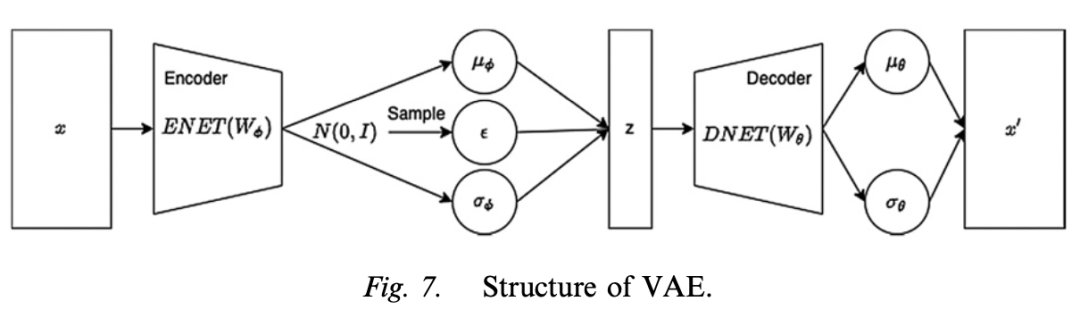
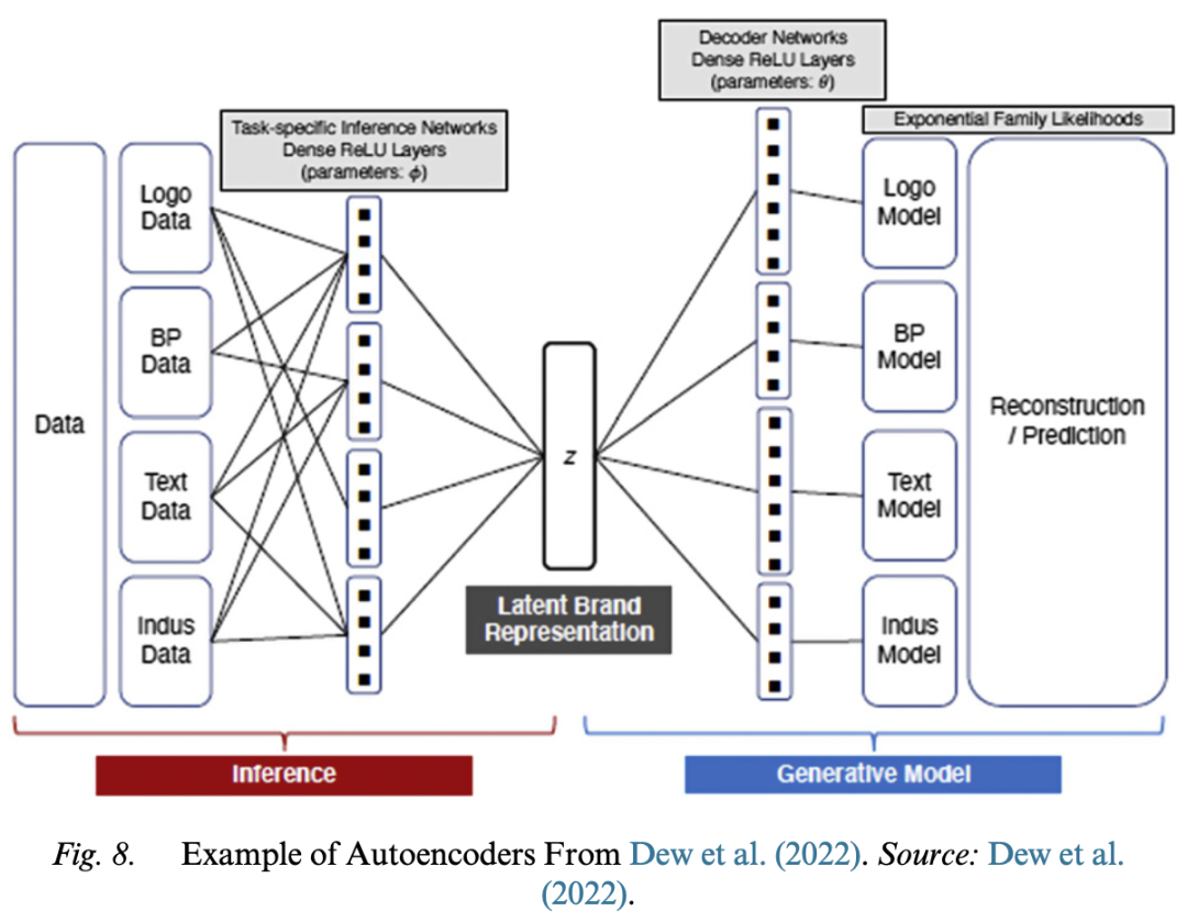
– **Model Mechanism**: VAE assumes that there exist some latent codes to explain the data generating process. It infers the latent codes from the input data and then uses the latent codes to generate new data with the same distribution as the input data. It is a combination of probabilistic graphical models and ANN and includes an encoder network and a decoder network.

– **Advantages and Disadvantages**: The advantages are that the latent space can be used to visualize and understand the structure of the input data; the disadvantages are that the generated images may be blurry.

– **Implementation Details**: Taking logo generation and car aesthetic design as examples, the application of VAE is introduced, involving the adjustment of multiple hyperparameters.

• Variational Autoencoders (VAE)

• Model Mechanism: VAE assumes that there exist some latent codes to explain the data generating process. It infers the latent codes from the input data and then uses the latent codes to generate new data with the same distribution as the input data. It is a combination of probabilistic graphical models and ANN and includes an encoder network and a decoder network.

• Advantages and Disadvantages: The advantages are that the latent space can be used to visualize and understand the structure of the input data; the disadvantages are that the generated images may be blurry.

• Implementation Details: Taking logo generation and car aesthetic design as examples, the application of VAE is introduced, involving the adjustment of multiple hyperparameters.

import tensorflow as tf
from tensorflow.keras import layers, models
from tensorflow.keras.losses import binary_crossentropy
import numpy as np
# Define sampling layer
class Sampling(layers.Layer):
    def call(self, inputs):
        z_mean, z_log_var = inputs
        batch = tf.shape(z_mean)[0]
        dim = tf.shape(z_mean)[1]
        epsilon = tf.keras.backend.random_normal(shape=(batch, dim))
        return z_mean + tf.exp(0.5 * z_log_var) * epsilon
# Define encoder
def build_encoder(input_shape, latent_dim):
    inputs = layers.Input(shape=input_shape)
    x = layers.Flatten()(inputs)
    x = layers.Dense(512, activation='relu')(x)
    x = layers.Dense(256, activation='relu')(x)
    z_mean = layers.Dense(latent_dim, name='z_mean')(x)
    z_log_var = layers.Dense(latent_dim, name='z_log_var')(x)
    z = Sampling()([z_mean, z_log_var])
    encoder = models.Model(inputs, [z_mean, z_log_var, z], name='encoder')
    return encoder
# Define decoder
def build_decoder(latent_dim, original_shape):
    latent_inputs = layers.Input(shape=(latent_dim,))
    x = layers.Dense(256, activation='relu')(latent_inputs)
    x = layers.Dense(512, activation='relu')(x)
    x = layers.Dense(np.prod(original_shape), activation='sigmoid')(x)
    outputs = layers.Reshape(original_shape)(x)
    decoder = models.Model(latent_inputs, outputs, name='decoder')
    return decoder
# Define VAE model
class VAE(models.Model):
    def __init__(self, encoder, decoder, **kwargs):
        super(VAE, self).__init__(**kwargs)
        self.encoder = encoder
        self.decoder = decoder
    def call(self, inputs):
        z_mean, z_log_var, z = self.encoder(inputs)
        reconstructed = self.decoder(z)
        kl_loss = -0.5 * tf.reduce_mean(
            z_log_var - tf.square(z_mean) - tf.exp(z_log_var) + 1)
        self.add_loss(kl_loss)
        return reconstructed
# Assume input shape is (28, 28, 1), latent dimension is 2
input_shape = (28, 28, 1)
latent_dim = 2
encoder = build_encoder(input_shape, latent_dim)
decoder = build_decoder(latent_dim, input_shape)
vae = VAE(encoder, decoder)
# Compile model
vae.compile(optimizer='adam', loss=binary_crossentropy)
# Print model summary
vae.encoder.summary()
vae.decoder.summary()

– **Generative Adversarial Networks (GAN)**

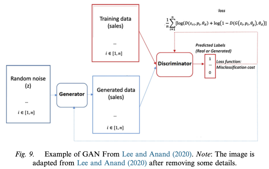
– **Model Mechanism**: GAN is based on a game-theory scenario with two adversarial players: a generator and a discriminator. The generator’s task is to generate data samples similar to the training data, and the discriminator’s task is to distinguish between real and fake samples.

– **Advantages and Disadvantages**: The advantages are that it performs well in generating realistic images; the disadvantages are that the learning process is difficult and it is not suitable for generating discrete data.

– **Implementation Details**: Common problems and solutions in training GAN are introduced, such as gradient explosion/vanishing and mode collapse.

• Generative Adversarial Networks (GAN)

• Model Mechanism: GAN is based on a game-theory scenario with two adversarial players: a generator and a discriminator. The generator’s task is to generate data samples similar to the training data, and the discriminator’s task is to distinguish between real and fake samples.

• Advantages and Disadvantages: The advantages are that it performs well in generating realistic images; the disadvantages are that the learning process is difficult and it is not suitable for generating discrete data.

• Implementation Details: Common problems and solutions in training GAN are introduced, such as gradient explosion/vanishing and mode collapse.

import tensorflow as tf
from tensorflow.keras import layers, models
# Define generator
def build_generator(latent_dim):
    model = models.Sequential()
    model.add(layers.Dense(256, activation='relu', input_dim=latent_dim))
    model.add(layers.BatchNormalization())
    model.add(layers.Dense(512, activation='relu'))
    model.add(layers.BatchNormalization())
    model.add(layers.Dense(1024, activation='relu'))
    model.add(layers.BatchNormalization())
    model.add(layers.Dense(28 * 28 * 1, activation='tanh'))
    model.add(layers.Reshape((28, 28, 1)))
    return model
# Define discriminator
def build_discriminator(input_shape):
    model = models.Sequential()
    model.add(layers.Flatten(input_shape=input_shape))
    model.add(layers.Dense(512, activation='relu'))
    model.add(layers.Dense(256, activation='relu'))
    model.add(layers.Dense(1, activation='sigmoid'))
    return model
# Define GAN model
class GAN(models.Model):
    def __init__(self, generator, discriminator, latent_dim, **kwargs):
        super(GAN, self).__init__(**kwargs)
        self.generator = generator
        self.discriminator = discriminator
        self.latent_dim = latent_dim
    def compile(self, d_optimizer, g_optimizer, loss_fn):
        super(GAN, self).compile()
        self.d_optimizer = d_optimizer
        self.g_optimizer = g_optimizer
        self.loss_fn = loss_fn
    def train_step(self, real_images):
        batch_size = tf.shape(real_images)[0]
        random_latent_vectors = tf.random.normal(shape=(batch_size, self.latent_dim))
        generated_images = self.generator(random_latent_vectors)
        combined_images = tf.concat([generated_images, real_images], axis=0)
        labels = tf.concat([tf.zeros((batch_size, 1)), tf.ones((batch_size, 1))], axis=0)
        labels += 0.05 * tf.random.uniform(tf.shape(labels))
        with tf.GradientTape() as tape:
            predictions = self.discriminator(combined_images)
            d_loss = self.loss_fn(labels, predictions)
        grads = tape.gradient(d_loss, self.discriminator.trainable_weights)
        self.d_optimizer.apply_gradients(zip(grads, self.discriminator.trainable_weights))
        misleading_labels = tf.ones((batch_size, 1))
        with tf.GradientTape() as tape:
            predictions = self.generator(random_latent_vectors)
            predictions = self.discriminator(predictions)
            g_loss = self.loss_fn(misleading_labels, predictions)
        grads = tape.gradient(g_loss, self.generator.trainable_weights)
        self.g_optimizer.apply_gradients(zip(grads, self.generator.trainable_weights))
        return {"d_loss": d_loss, "g_loss": g_loss}
# Hyperparameter settings
latent_dim = 100
input_shape = (28, 28, 1)
# Build generator and discriminator
generator = build_generator(latent_dim)
discriminator = build_discriminator(input_shape)
# Build GAN model
gan = GAN(generator=generator, discriminator=discriminator, latent_dim=latent_dim)
# Compile GAN model
gan.compile(
    d_optimizer=tf.keras.optimizers.Adam(learning_rate=0.0003),
    g_optimizer=tf.keras.optimizers.Adam(learning_rate=0.0003),
    loss_fn=tf.keras.losses.BinaryCrossentropy())
# Print model summary
generator.summary()
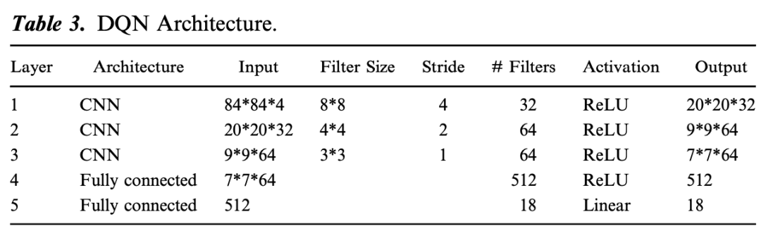
discriminator.summary()

– **Reinforcement Learning (RL) Models (Deep Q – Network, DQN)**

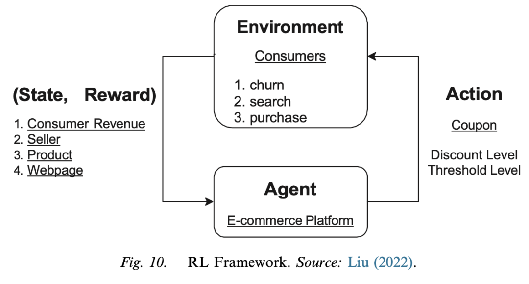
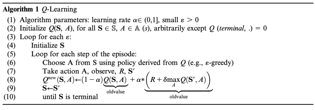
– **Model Mechanism**: RL solves sequential decision-making problems. DQN combines DL and RL and is used to handle high-dimensional problems. Taking the targeted distribution of coupons in live-stream shopping as an example, the Markov decision process (MDP) framework of RL is introduced, including elements such as state space, action space, rewards, etc., and how to learn the optimal policy through the Q – Learning algorithm.

– **Advantages and Disadvantages**: The advantages are that it can directly use high-dimensional input and outperform humans in difficult decision-making problems; the disadvantages are that it can only handle low-dimensional, discrete action spaces.

– **Implementation Details**: The original model architecture of DQN and two techniques for achieving stable convergence (experience replay and adding a target network) are introduced, as well as the specific settings in marketing applications.

• Reinforcement Learning (RL) Models (Deep Q – Network, DQN)

• Model Mechanism: RL solves sequential decision-making problems. DQN combines DL and RL and is used to handle high-dimensional problems. Taking the targeted distribution of coupons in live-stream shopping as an example, the Markov decision process (MDP) framework of RL is introduced, including elements such as state space, action space, rewards, etc., and how to learn the optimal policy through the Q – Learning algorithm.

• Advantages and Disadvantages: The advantages are that it can directly use high-dimensional input and outperform humans in difficult decision-making problems; the disadvantages are that it can only handle low-dimensional, discrete action spaces.

• Implementation Details: The original model architecture of DQN and two techniques for achieving stable convergence (experience replay and adding a target network) are introduced, as well as the specific settings in marketing applications.

import numpy as np
import tensorflow as tf
from tensorflow.keras import layers, models
from collections import deque
import random
# Define DQN model
def build_dqn_model(state_shape, action_size):
    model = models.Sequential()
    model.add(layers.Dense(24, input_shape=state_shape, activation='relu'))
    model.add(layers.Dense(24, activation='relu'))
    model.add(layers.Dense(action_size, activation='linear'))
    return model
# Define DQN agent
class DQNAgent:
    def __init__(self, state_shape, action_size):
        self.state_shape = state_shape
        self.action_size = action_size
        self.memory = deque(maxlen=2000)
        self.gamma = 0.95  # Discount factor
        self.epsilon = 1.0  # Exploration rate
        self.epsilon_min = 0.01
        self.epsilon_decay = 0.995
        self.learning_rate = 0.001
        self.model = build_dqn_model(state_shape, action_size)
        self.target_model = build_dqn_model(state_shape, action_size)
        self.update_target_model()
    def update_target_model(self):
        self.target_model.set_weights(self.model.get_weights())
    def remember(self, state, action, reward, next_state, done):
        self.memory.append((state, action, reward, next_state, done))
    def act(self, state):
        if np.random.rand() <= self.epsilon:
            return random.randrange(self.action_size)
        act_values = self.model.predict(state)
        return np.argmax(act_values[0])
    def replay(self, batch_size):
        minibatch = random.sample(self.memory, batch_size)
        for state, action, reward, next_state, done in minibatch:
            target = self.model.predict(state)
            if done:
                target[0][action] = reward
            else:
                t = self.target_model.predict(next_state)[0]
                target[0][action] = reward + self.gamma * np.amax(t)
            self.model.fit(state, target, epochs=1, verbose=0)
        if self.epsilon > self.epsilon_min:
            self.epsilon *= self.epsilon_decay
    def load(self, name):
        self.model.load_weights(name)
    def save(self, name):
        self.model.save_weights(name)
# Assume state space is (4,) action space size is 2
state_shape = (4,)
action_size = 2
agent = DQNAgent(state_shape, action_size)
# Train DQN agent
def train_dqn(agent, env, episodes, batch_size):
    for e in range(episodes):
        state = env.reset()
        state = np.reshape(state, [1, state_shape[0]])
        for time in range(500):
            action = agent.act(state)
            next_state, reward, done, _ = env.step(action)
            reward = reward if not done else -10
            next_state = np.reshape(next_state, [1, state_shape[0]])
            agent.remember(state, action, reward, next_state, done)
            state = next_state
            if done:
                agent.update_target_model()
                print(f"episode: {e}/{episodes}, score: {time}, e: {agent.epsilon:.2}")
                break
            if len(agent.memory) > batch_size:
                agent.replay(batch_size)
# Example environment and training parameters
# env = gym.make('CartPole-v1')  # Example environment
# train_dqn(agent, env, episodes=1000, batch_size=32

### 5. How DL Helps Solve Marketing Problems

– **Plug and Play**

– When a marketing problem involves unstructured data, an off-the-shelf DL algorithm can be used to process the data, extract an interpretable numerical variable, and then use the variable in subsequent analysis, such as for designing experimental stimuli or as an independent or dependent variable in an econometrics model.

• Plug and Play

• When a marketing problem involves unstructured data, an off-the-shelf DL algorithm can be used to process the data, extract an interpretable numerical variable, and then use the variable in subsequent analysis, such as for designing experimental stimuli or as an independent or dependent variable in an econometrics model.

– **Customized Algorithm Development**

– **Combining Unstructured Data with Structured Data**: The marketing environment is complex, and the output of DL prediction often needs to be combined with other variables from structured data to explain or predict a response variable. Structured data variables can be added to DNN, and the specific addition position can be determined according to domain knowledge.

– **Theory-Driven Architecture Design**: Existing theories can guide the choice of DNN architecture. For example, the CNN architecture originates from theories in the visual pattern recognition literature. The interaction theories of social psychology and economics in marketing research can also provide information for the architecture design of marketing problems.

• Combining Unstructured Data with Structured Data

• The marketing environment is complex, and the output of DL prediction often needs to be combined with other variables from structured data to explain or predict a response variable. Structured data variables can be added to DNN, and the specific addition position can be determined according to domain knowledge.

• Theory-Driven Architecture Design

• Existing theories can guide the choice of DNN architecture. For example, the CNN architecture originates from theories in the visual pattern recognition literature. The interaction theories of social psychology and economics in marketing research can also provide information for the architecture design of marketing problems.

– **Theory-Driven Initialization**: The training process of DL models is iterative, and the choice of initialization affects the convergence speed. Marketing theories can guide the parameter initialization of DL models like providing prior information for Bayesian models.

– **Customized Constraints**: Each specific marketing environment may impose additional constraints on DL models. For example, combining the VAE/GAN model with masks to generate car images that meet specific shape requirements.

• Theory-Driven Initialization

• The training process of DL models is iterative, and the choice of initialization affects the convergence speed. Marketing theories can guide the parameter initialization of DL models like providing prior information for Bayesian models.

• Customized Constraints

• Each specific marketing environment may impose additional constraints on DL models. For example, combining the VAE/GAN model with masks to generate car images that meet specific shape requirements.

### 6. Conclusion and Future Research Directions

– **Conclusion**: DL provides tools for marketers to analyze large-scale and unstructured data, expanding the scope of marketing research. Discriminative DL models can extract important factors from unstructured data, generative DL models can assist in content production and creative design, and reinforcement learning enables marketers to develop optimal dynamic strategies.

• DL provides tools for marketers to analyze large-scale and unstructured data, expanding the scope of marketing research. Discriminative DL models can extract important factors from unstructured data, generative DL models can assist in content production and creative design, and reinforcement learning enables marketers to develop optimal dynamic strategies.

– **Future Research Directions**

– **Multimodal, Five Senses, and Networks**: Marketing content is increasingly multimodal. In the future, it is expected to use DL to expand from two senses (visual and auditory) to five senses and process network data.

– **Model Efficiency Improvement**: Existing DL requires a large amount of labeled data, and there are problems with the computing power required to run the models. In the future, by utilizing the marketing system structure and choosing more appropriate model architectures, the demand for labeled data and computing costs can be reduced.

• Multimodal, Five Senses, and Networks

• Marketing content is increasingly multimodal. In the future, it is expected to use DL to expand from two senses (visual and auditory) to five senses and process network data.

• Model Efficiency Improvement

• Existing DL requires a large amount of labeled data, and there are problems with the computing power required to run the models. In the future, by utilizing the marketing system structure and choosing more appropriate model architectures, the demand for labeled data and computing costs can be reduced.

– **Reinforcement Learning**: Most DL applications in marketing focus on system 1 tasks, while marketing interventions are mainly system 2 tasks. There is great development space for reinforcement learning in this regard.

– **Causal Inference**: DL can be used not only for predictive and generative tasks but also for causal inference. In the future, more deep causal inferences in marketing applications are expected, including various estimation methods and solutions to endogeneity problems.

– **Common Testbeds**: The marketing community needs to establish datasets representing common marketing problems as common testbeds to promote the development and progress of algorithms.

• Reinforcement Learning

• Most DL applications in marketing focus on system 1 tasks, while marketing interventions are mainly system 2 tasks. There is great development space for reinforcement learning in this regard.

• Causal Inference

• DL can be used not only for predictive and generative tasks but also for causal inference. In the future, more deep causal inferences in marketing applications are expected, including various estimation methods and solutions to endogeneity problems.

• Common Testbeds

• The marketing community needs to establish datasets representing common marketing problems as common testbeds to promote the development and progress of algorithms.