
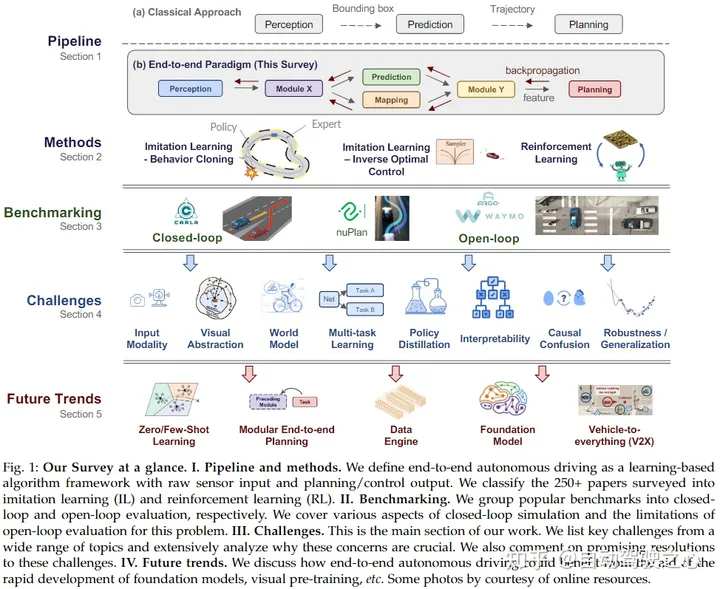
Introduction
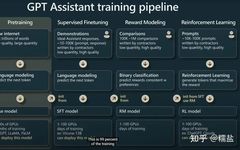
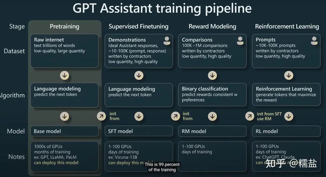
Tesla’s FSD has popularized self-supervised learning, and large models like GPT also utilize the concept of self-supervised learning. As we know, the cost of supervised learning is prohibitively high, especially for complex tasks, such as FSD systems. Tesla has collected training data exceeding 400 million kilometers, and without the help of an “automated labeling system,” this data would be practically unusable for training. Even with Tesla’s own Dojo supercomputer and a complete set of automated data closed-loop systems for labeling and training software, data labeling and training cannot be completed quickly enough because labeling will always become the bottleneck of the data closed loop. It relies on larger networks and extensive software for cleaning and correction, consuming vast computing power, bandwidth, and storage, and occasionally requiring some manual intervention, interrupting the cycle. Looking at the training steps of ChatGPT, the first column is Pre-training, which accounts for 99% of the training dataset, while the second, third, and fourth columns are tasks that contractors need to perform, generating or labeling data that only accounts for 1% or less.
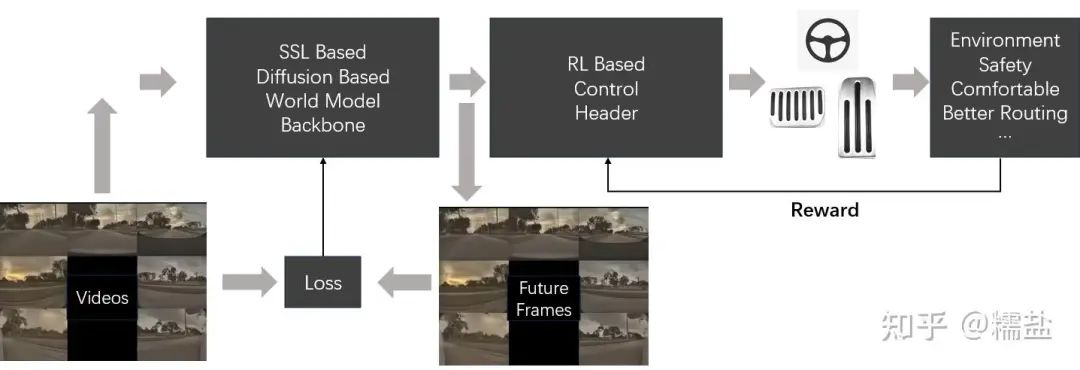
At CVPR 2023, Tesla showcased their so-called “General World Model,” clearly stating that this world model can predict the future, can be controlled, can generate different forms of output, can be used for simulation, and can generate rare situations. This indirectly represents that self-supervised learning has become the backbone network for the entire FSD version 12.0. After 400 million kilometers of video self-supervised learning training, this model has surpassed the previous “large perception” versions, enabling it to understand the operational laws of the physical world. The model can be roughly described as follows:
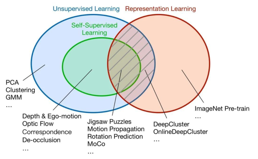
Self-Supervised Learning, also known as self-supervised learning, is a popular research area in recent years. We know that general machine learning is divided into supervised learning, unsupervised learning, and reinforcement learning. Self-supervised learning is a type of unsupervised learning that aims to learn a general feature representation for downstream tasks.

1. What is Self-Supervised Learning
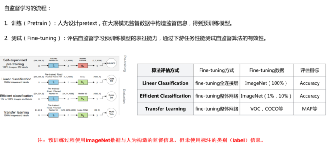
In deep learning-based models, we usually first extract features from data using a backbone network, such as VGG, ResNet, MobileNet, and Inception, and then feed the extracted feature maps into downstream tasks like classification, detection, or segmentation. The backbone is effective because it has been pre-trained on datasets like ImageNet, thus possessing strong feature extraction capabilities. Here, a large labeled dataset (like ImageNet) is crucial, but when facing a new domain or task without a large amount of labeled data, self-supervised learning becomes very important:
Self-supervised learning is a relatively hot research area in the past two years, aiming to extract the representation characteristics of unlabeled data by designing proxy tasks as supervisory information to enhance the model’s feature extraction capability (Note: the supervisory information obtained here does not refer to the original task labels faced by self-supervised learning, but rather the constructed proxy task labels). Pay attention to the two keywords here: unlabeled data and auxiliary information, which are the two key bases for defining self-supervised learning.
Since we mentioned self-supervised learning, let’s also briefly introduce several types of learning:
Supervised Learning: Supervised learning learns a function (model parameters) from a given labeled training dataset, which can predict results based on this function when inputting new test data;
Unsupervised Learning: Unsupervised learning analyzes the regularities and characteristics of data from unlabeled data. Unsupervised learning algorithms can be divided into two main categories: methods based on probability density function estimation and methods based on similarity measures between samples;
Semi-supervised Learning: Semi-supervised learning lies between supervised and unsupervised learning, where only a portion of the training set has labels, and model training needs to be completed through methods like pseudo-label generation;
Weakly-supervised Learning: Weakly-supervised learning refers to training data that only has imprecise or incomplete label information, such as in object detection tasks where the training data only contains category labels without bounding box coordinate information.
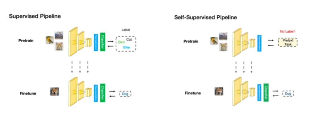
1.1 Differences Between Self-Supervised and Supervised Learning
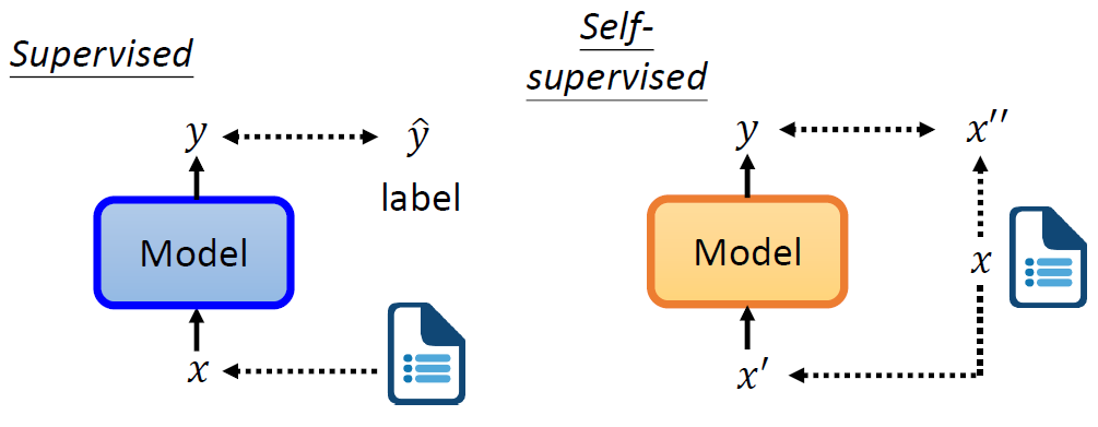
As shown in the figure below, when we previously performed supervised learning, how did we let the model output the desired y? You must have labeled data. Suppose we want to perform sentiment analysis, where the machine looks at a piece of text and outputs whether the sentiment is positive or negative. You need a large collection of articles with corresponding labels to train the model.
Self-supervised learning, on the other hand, finds a way to supervise itself without labels. We still have the same set of data x, which we now divide into two parts: x′ and x′′. Then, we input x′ into the model and let it output y, and we want y to be as close as possible to x′′, which is self-supervised learning. In other words, in self-supervised learning, one part of the input serves as a supervisory signal, while the other part remains as input.
Self-supervised learning constructs representations by learning to encode the similarity or dissimilarity between two entities, i.e., by constructing positive and negative samples and measuring the distance between them. The core idea is that the similarity between samples and positive samples is far greater than that between samples and negative samples, similar to the triplet model.
Based on different pretext pre-training methods designed by humans, self-supervised learning can be divided into the following three categories:
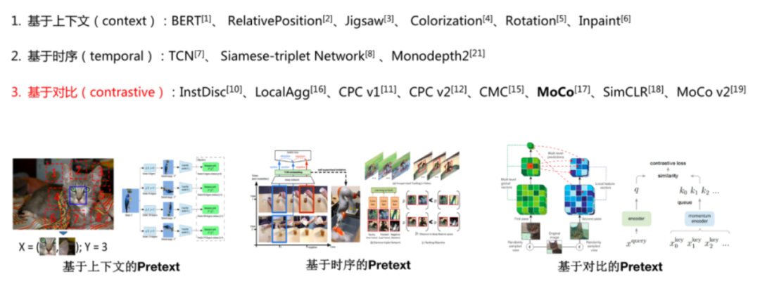
1.2 Context-Based
1.2.1 Context-Based Pre-training in NLP
The order of sentences has strong regularity, so sequential information is key to designing auxiliary tasks in natural language processing tasks. For NLP, it mainly follows a Pretrain-Finetune pattern. Let’s first review the Pretrain-Finetune process in supervised learning: we first train on a large amount of labeled data to obtain a pre-trained model, then for new downstream tasks, we transfer the learned parameters and fine-tune them on new labeled tasks to obtain a network that can adapt to the new task. In self-supervised learning, the Pretrain-Finetune process starts with a large amount of unlabeled data to train the network through pretext tasks to obtain a pre-trained model, then for new downstream tasks, just like in supervised learning, fine-tune the transferred parameters. Therefore, the capability of self-supervised learning is mainly reflected in the performance of downstream tasks. This is also the operation of fine-tuning large models.
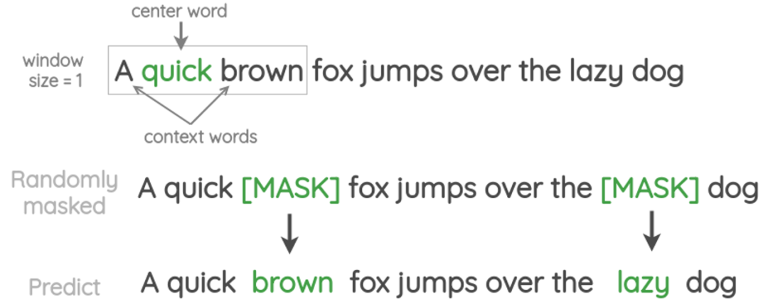
a. Word Prediction —- This type actually uses the original dialogue as the ground truth to calculate loss.
The most common method is to randomly delete words from sentences in the training set to construct auxiliary task training sets and labels to train the network to predict the deleted words, enhancing the model’s ability to extract sequential features (BERT).
1.2.2 Context-Based for Images
a. Image Reassembly (Jigsaw Puzzles) —- In this case, the ground truth is the original image to calculate loss.
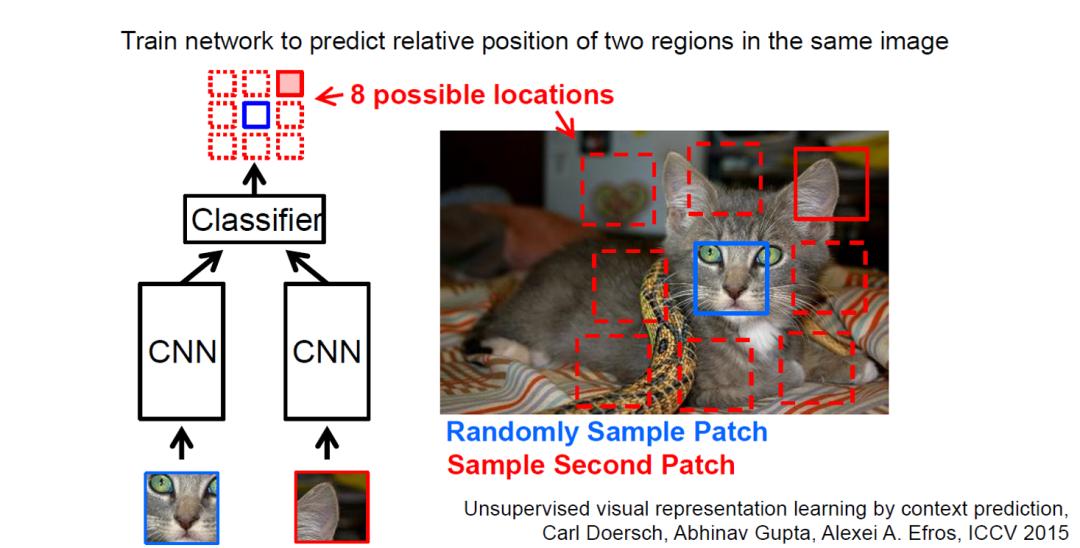
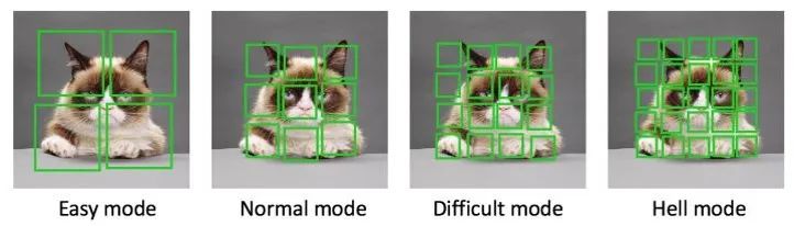
In images, researchers have constructed auxiliary tasks using a method called Jigsaw (puzzles). We can divide an image into 9 parts and then predict the relative positions of these parts to generate loss. For example, if we input the cat’s eyes and right ear from this image, we expect the model to learn that the cat’s right ear is above its face. If the model can perform this task well, we can conclude that the representation learned by the model contains semantic information.
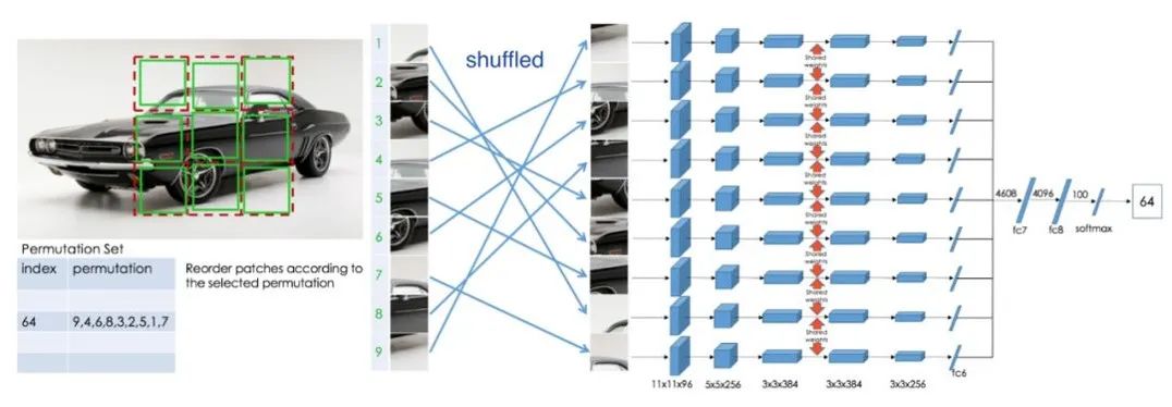
Subsequent work has expanded this puzzle method, designing more complex or difficult tasks. First, we still divide the image into 9 pieces, and we predefine 64 sorting methods. The model inputs any disordered sequence and learns to identify which class the order belongs to. Compared to the previous work, this model needs to learn more relative positional information. The insight gained from this work is that using stronger supervisory information, or making auxiliary tasks more challenging, leads to better final performance.
b. Image Colorization
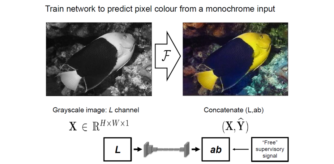
This involves converting RGB images in the original dataset to grayscale and training the network through the image color restoration task. By providing the model with the grayscale image, it predicts the color of the image. Only if the model can understand the semantic information in the image can it know what color each part should be, such as the sky being blue and the grass being green. The model must learn these semantic concepts from vast amounts of data to determine the specific color information of objects. After training, this model can perform the task of coloring images.
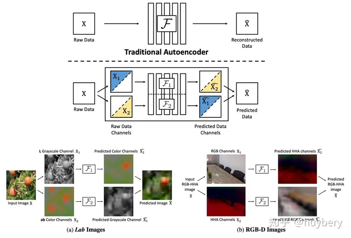
The color prediction model has provided new insights, as the grayscale image and the ab domain information can be regarded as a decoupled representation of an image. Therefore, any decoupled features can be learned through this mutual supervision approach. The well-known Split-Brain Autoencoders are doing just that. For the original data, it is first divided into two parts, and then one part’s information is used to predict the other part, resulting in a complete data synthesis.
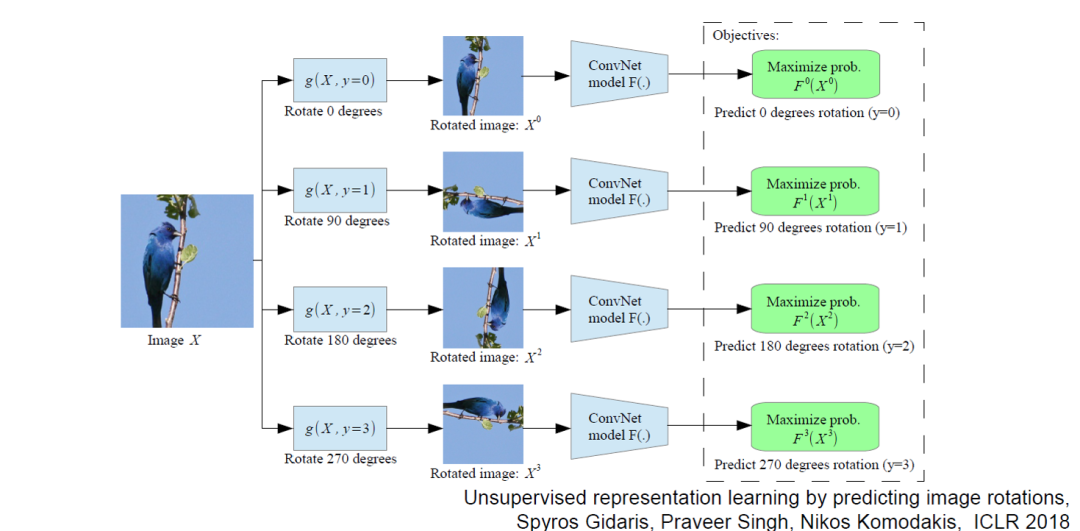
c. Image Rotation Angle Prediction
Randomly rotating images in the training set and training the network through a rotation angle regression task. The ICLR 2018 work involves giving an input image and rotating it at different angles, with the model’s goal being to predict the rotation angle of the image. This simple idea has led to significant gains, demonstrating that data augmentation is very beneficial for self-supervised learning. My personal view is that data augmentation not only provides more data but also enhances the robustness of pre-trained models.
d. Image Inpainting
The last method involves image segmentation. The idea is quite simple and straightforward: randomly remove a portion of the image and use the remaining part to predict the removed section. Only if the model truly understands what the image represents can it effectively complete the task. This work shows that self-supervised learning tasks can not only perform representation learning but also accomplish some remarkable tasks.
e. Multi-Task Learning
Combining the above auxiliary tasks to train the model.
Paper 1: “Rethinking Data Augmentation: Self-Supervision and Self-Distillation”
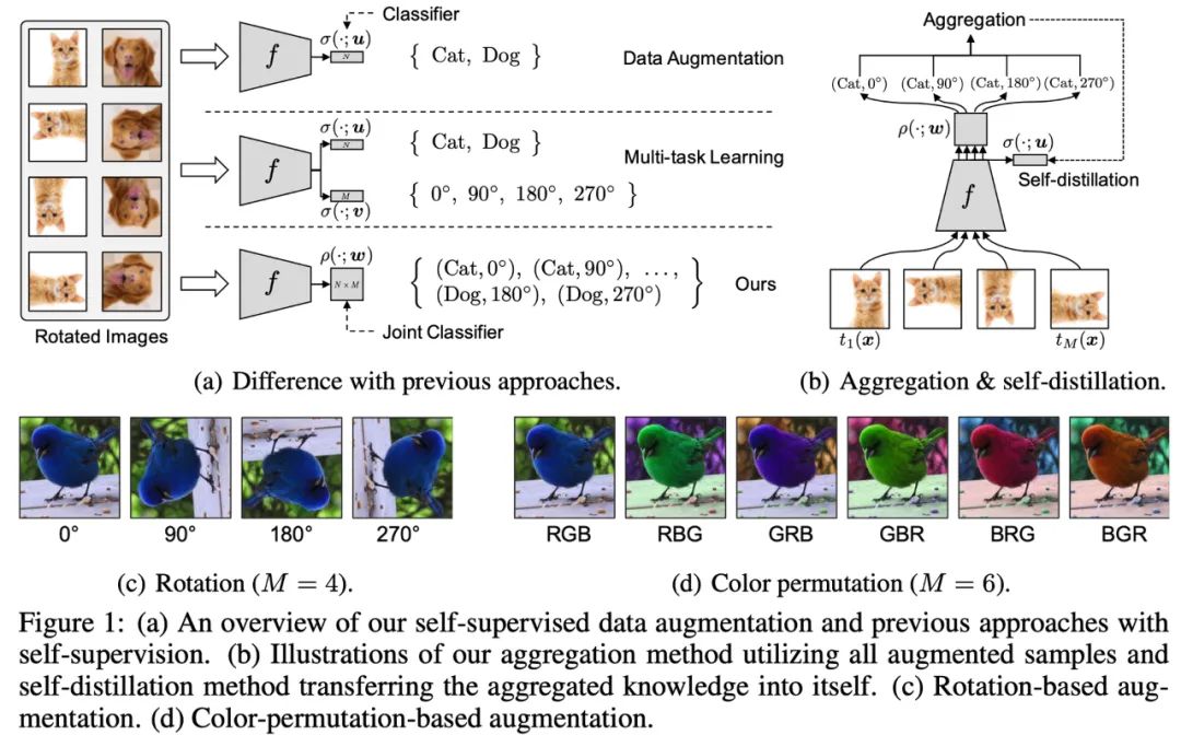
Methods related to data augmentation can expand the original training set by applying transformations (color, rotation, cropping, etc.) to improve model generalization.
Multi-task learning combines normal classification tasks with self-supervised learning tasks (like rotation prediction) to learn together.
The authors point out that learning through methods like data augmentation or multi-task learning can force features to have a certain invariance, making learning more difficult and potentially leading to performance degradation.
Therefore, the authors propose combining the categories of classification tasks and self-supervised learning tasks into more categories (e.g., (Cat, 0), (Cat, 90), etc.) using a single loss function for learning.
Paper 2: “S4L: Self-Supervised Semi-Supervised Learning”
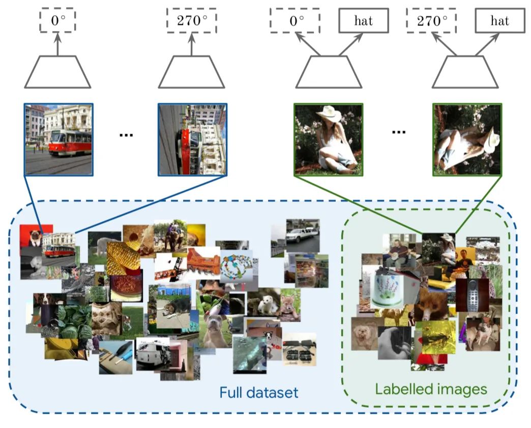
Self-supervised and semi-supervised learning (with a large amount of data without labels and a small amount with labels) can also be combined. Self-supervised learning (rotation prediction) is applied to unlabeled data, while for labeled data, supervised learning is conducted alongside self-supervised learning through joint training. By partitioning ImageNet into semi-supervised sets and experimenting with 10% or 1% of the data, the authors analyzed the impact of some hyperparameters on final performance.
For labeled data, the model simultaneously predicts the rotation angle and labels, while for unlabeled data, it only predicts the rotation angle. The prediction of the rotation angle can be replaced with any other unsupervised task (the authors proposed two algorithms: one is S^4L-Rotation, where the unsupervised loss is the rotation prediction task; the other is S^4L-Exemplar, where the unsupervised loss is based on image transformations (cropping, mirroring, color transformations, etc.) using triplet loss).
In summary, it is necessary to leverage unsupervised learning to create a pretext task for unlabeled data, enabling the model to learn a good feature representation from a large amount of unlabeled data.

2. Temporal Based
The methods introduced earlier are mostly based on the information of the samples themselves, such as rotation, color, cropping, etc. However, there are many constraints between samples, such as the similarity of adjacent frames in a video or multiple visual frames of an object.
2.1 NLP Temporal-Based —- In this case, the ground truth is the original dialogue to calculate loss
a. Sentence Sequence Prediction
b. Word Sequence Prediction

2.2 Image Temporal-Based —- In this case, the ground truth is the original video sequence to calculate loss
The previously introduced methods are mostly based on the information of the samples themselves, such as rotation, color, cropping, etc. However, there are many constraints between samples. Here, we introduce methods for self-supervised learning based on temporal constraints. The most representative data type for temporal constraints is video.
a. Similarity Based on Objects in Video
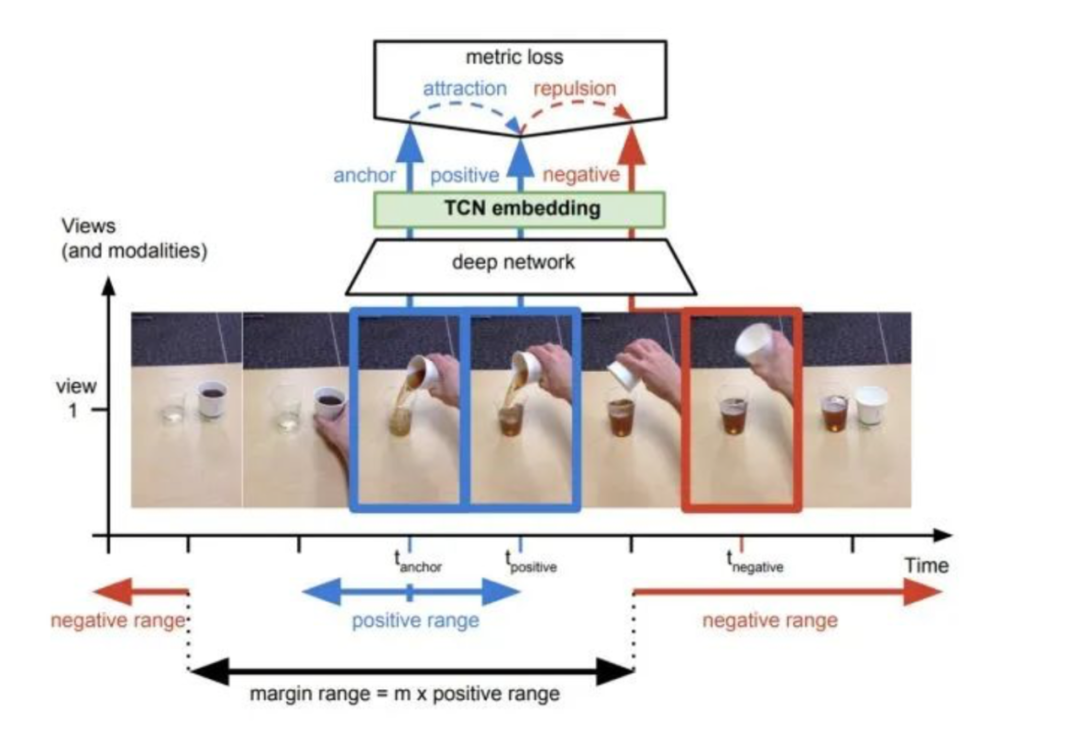
The first idea is based on frame similarity. For each frame in a video, there exists a concept of feature similarity. Simply put, we can consider that adjacent frames in a video have similar features, while frames that are far apart are dissimilar. By constructing positive (similar) and negative (dissimilar) samples, we can impose self-supervised constraints.
Paper 3: “Time-Contrastive Networks: Self-Supervised Learning from Video”
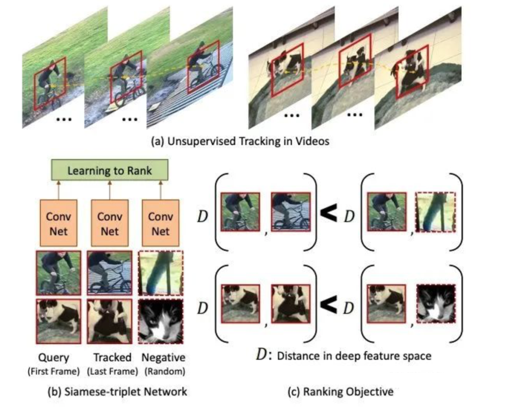
b. Unsupervised Object Tracking Based on Similarity
Capturing the same object from multiple viewpoints (multi-view) leads to the same frame having similar features, while different frames can be considered dissimilar. The network learns to discern the similarity of the same object and the dissimilarity of different objects across different frames to enhance feature extraction capabilities.
Paper 4: “Unsupervised Learning of Visual Representations Using Videos”
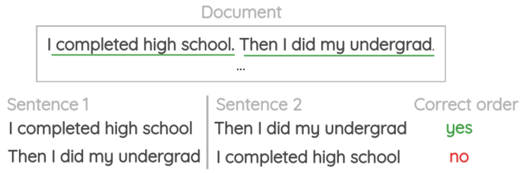
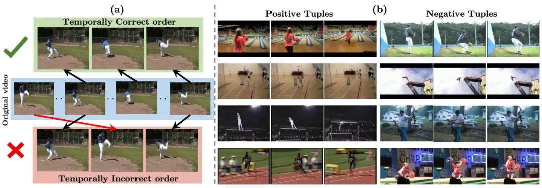
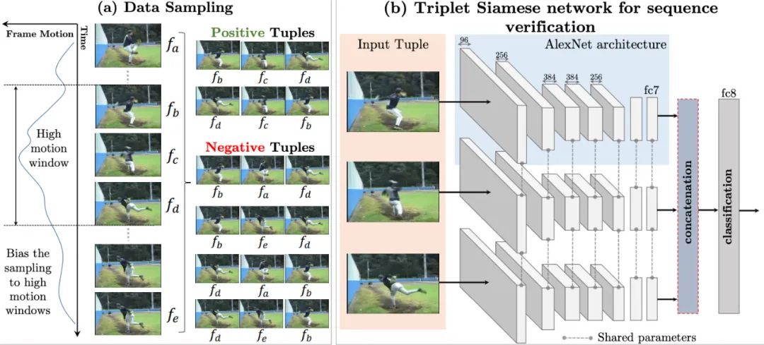
c. Sequence Information Based on Video Frames
This is quite similar to sequence prediction in natural language processing. We randomly shuffle the order of video frames in the training set to train the network to predict the correct video sequence. Methods based on order constraints can sample correct and incorrect video sequences from the video, constructing positive and negative sample pairs for training. In short, the goal is to design a model that can determine whether the current video sequence is in the correct order.
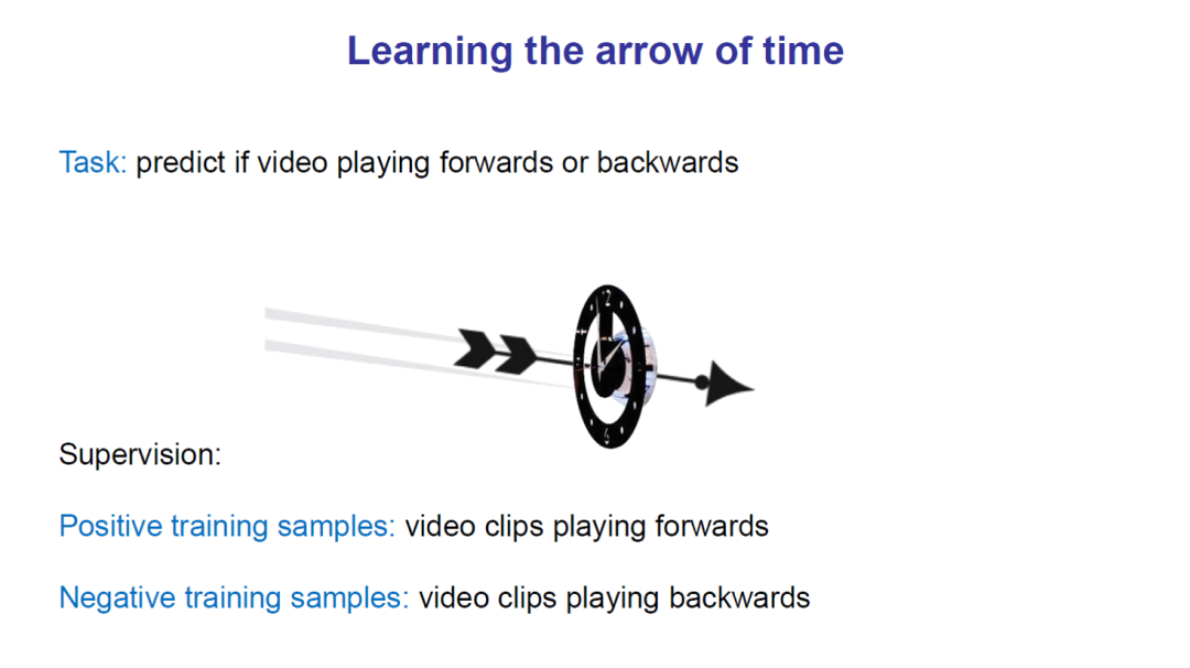
Paper 5: “Shuffle and learn: unsupervised learning using temporal order verification”
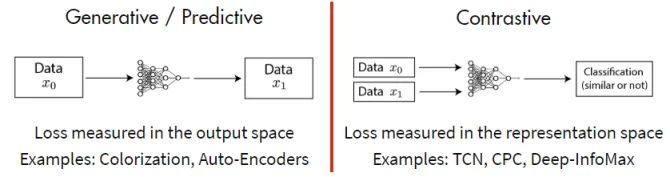
2.3 Contrastive Based —- In this case, the ground truth is whether two entities are similar to calculate loss
The third category of self-supervised learning methods is based on contrastive constraints. It constructs representations by learning to encode the similarity or dissimilarity between two entities. The performance of these methods is currently very strong, as evidenced by the recent focus of many experts in this direction. In fact, the temporal-based methods introduced in the second part already involve these contrastive constraints, by constructing positive and negative samples and measuring the distance between them to achieve self-supervised learning. The core idea is that the similarity between samples and positive samples is far greater than that between samples and negative samples:
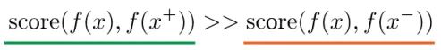
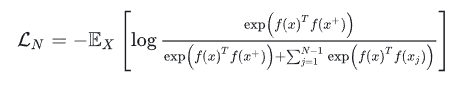
Here, x is often referred to as “anchor” data. To optimize the relationship between anchor data and its positive and negative samples, we can use a dot product to construct a distance function, and then create a softmax classifier to correctly classify positive and negative samples. This should encourage the similarity metric function (dot product) to assign larger values to positive examples and smaller values to negative examples:
Paper 6: “Learning deep representations by mutual information estimation and maximization”
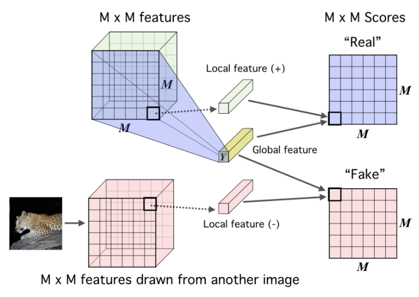
Deep InfoMax learns image representations by leveraging local structures within images. The contrastive task involves classifying global and local features within a pair of images.
Global features are the final outputs of a CNN, while local features are the outputs from intermediate layers of the encoder. Each local feature map has a limited receptive field.
For an anchor image x, f(x) is the global feature from one image, while the positive sample f(x+) is a local feature from the same image, and the negative sample f(x−) is a local feature from a different image.
The simple idea explored in this paper is to train a representation learning function, i.e., an encoder, to maximize the mutual information (MI) between its input and output. The authors combine MI maximization and prior matching in a manner similar to adversarial autoencoders, constraining representations according to desired statistical properties.
To obtain a representation more suitable for classification, the authors maximize the average MI value between the high-level representation of the image and local patches.
Paper 7: “Representation Learning with Contrastive Predictive Coding”
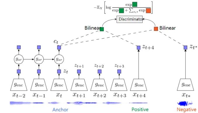
CPC is a contrastive-based self-supervised framework that can be applied to any form of data, including text, speech, video, and images (where images can be viewed as sequences of pixels or image blocks).
CPC learns feature representations by encoding information shared across multiple time points while discarding local information. These features are referred to as “slow features”: characteristics that do not change rapidly over time, such as the identity of a speaker in a video, activities in a video, or objects in an image.
CPC primarily utilizes an autoregressive approach to learn representations by encoding shared information between data points separated by multiple time steps. This representation ct can represent information fused from the past, while the positive sample is the input after time t, and the negative sample is randomly sampled from other sequences. The main idea of CPC is to predict future data based on past information through a sampling method.
Paper 8: “Momentum Contrast for Unsupervised Visual Representation Learning”
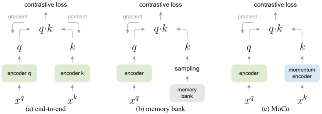
Contrastive self-supervised learning involves training an encoder to ensure similarity with corresponding keys in a larger dictionary, while being dissimilar to others.
Traditionally, the dictionary size is equal to the batch size. Due to computational limitations, it cannot be set too large, making it difficult to apply a large number of negative samples, resulting in low efficiency.
This paper proposes to use a queue to store this dictionary. During training, each new batch is encoded and enters the queue, while the oldest batch’s key exits the queue. This way, the size of the dictionary can be much larger than the batch size, greatly increasing the number of negative samples and improving efficiency.
a. Traditional Method – End-to-End. In this approach, queries and keys use two encoders, and both parameters are updated. However, this method limits the dictionary size to the mini-batch size.
b. Using a larger memory bank to store a larger dictionary (storing all samples), but only updating the memory after each query, resulting in potentially outdated vectors being queried, which can lose consistency.
c. Using a queue, where the oldest batch’s samples are removed after each query, and the latest batch is updated into the queue. This cleverly alleviates the memory bank consistency issue. At the same time, using a queue allows for storing many more samples than the batch size, solving the coupling problem of end-to-end batch size.
Paper 9: “A Simple Framework for Contrastive Learning of Visual Representations”
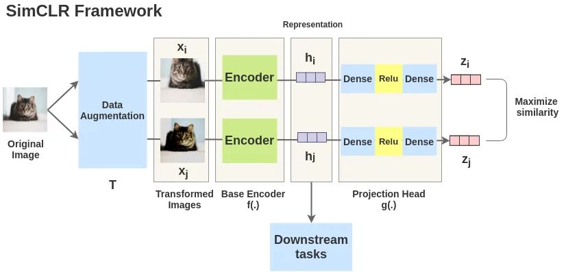
Take an image and apply random transformations to obtain a pair of augmented images xi and xj. Each image in this pair is encoded to obtain its representation. Then, a nonlinear fully connected layer is used to obtain the representations z, with the task being to maximize the similarity between zi and zj.
The random data augmentation module involves random cropping followed by resizing to the same size, along with random color perturbation and random Gaussian blur. The combination of random cropping and color perturbation is crucial for achieving good performance.
The neural network base encoder is used to extract representation vectors from augmented data samples. This framework can be applied to different network architectures without restrictions. The authors use a simple, general ResNet.
The neural network projection head g() maps the representation to the space where contrastive loss is applied.
The contrastive loss function is used for the contrastive prediction task. Given a dataset containing positive sample pairs, the goal of the contrastive prediction task is to identify the positive sample pairs.

3. End-to-End Self-Supervised Autonomous Driving
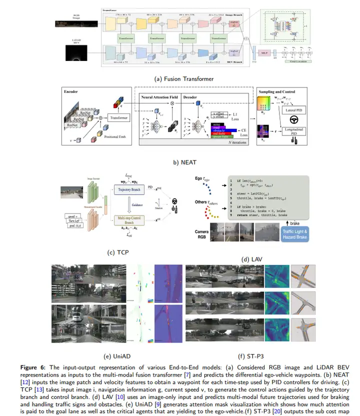
Let’s not forget the core of this article——-end-to-end self-supervised driving. This is also to be achieved through methods like the World Model for end-to-end autonomous driving. In the field of autonomous driving, end-to-end driving strategy learning takes raw sensor data (images, vehicle signals, point clouds, etc.) as input and directly predicts control signals or plans routes. Due to the complexity and uncertainty of the driving environment, as well as the large amount of irrelevant information in sensor data, learning an end-to-end driving strategy model from scratch is challenging, often requiring a large amount of labeled data or environmental interaction feedback to achieve satisfactory performance.
A typical end-to-end autonomous driving system is illustrated as follows:
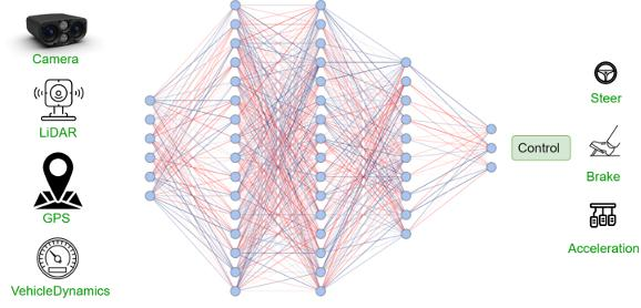
Input: Most autonomous vehicles are equipped with various sensors, including cameras, Lidar, and millimeter-wave radar, which collect data from these sensors and input it into deep learning systems.
Output: The system can directly output control signals such as steering angles, throttle, and brake, or it can first output trajectories and then convert these trajectories into steering angles, throttle, and brake signals based on different vehicle dynamics models.
It can be seen that the end-to-end autonomous driving system functions like the human brain, receiving information through sensors like eyes and ears, processing it, and then issuing commands to execute actions. However, this simplicity also hides significant risks, such as poor explainability, as it cannot analyze intermediate results like traditional autonomous driving tasks; it requires high-quality, diverse, and massive training data; otherwise, AI will face the garbage in, garbage out problem.
Traditional autonomous driving is task-specific, necessarily involving multiple modules. End-to-end autonomous driving can be achieved with a single module, though it can also be implemented with multiple modules, differing in whether it is trained end-to-end. In a task-specific system, each task is trained, optimized, and evaluated independently, while in an end-to-end system, all modules are treated as a whole for end-to-end training and evaluation.
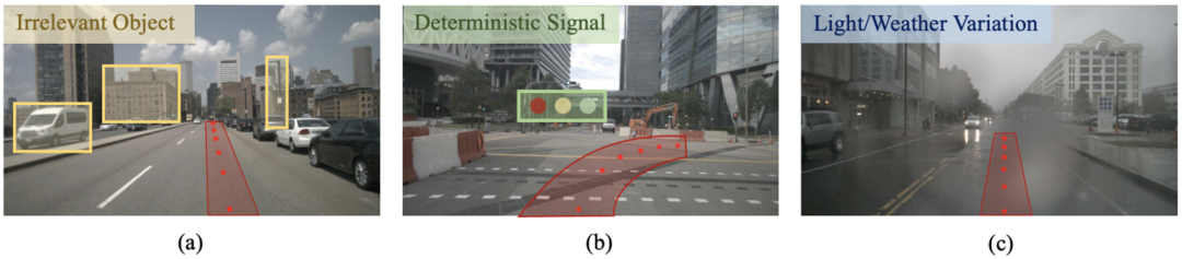
In the natural environment, there is much information that does not need attention, such as buildings, weather changes, and lighting variations. For the driving task, the critical information to focus on is where to drive next and whether traffic lights allow passage.
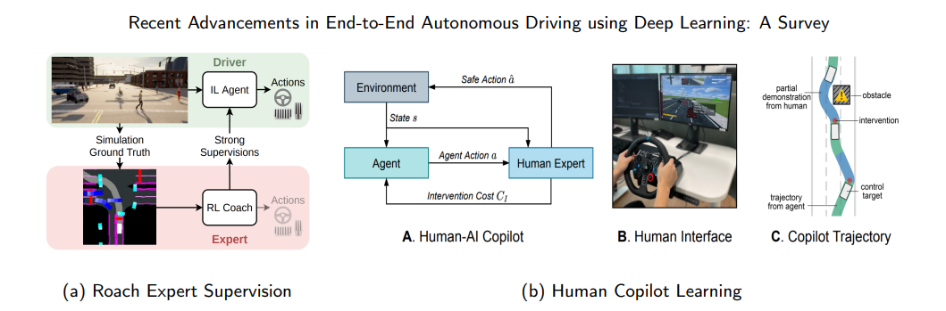
3.1 Imitation Learning (IL)
Based on the principle of learning from expert demonstrations. These demonstrations train the system to mimic expert behavior in various driving scenarios. Large-scale expert driving datasets are readily available and can be used to train models that meet human standards through imitation learning.
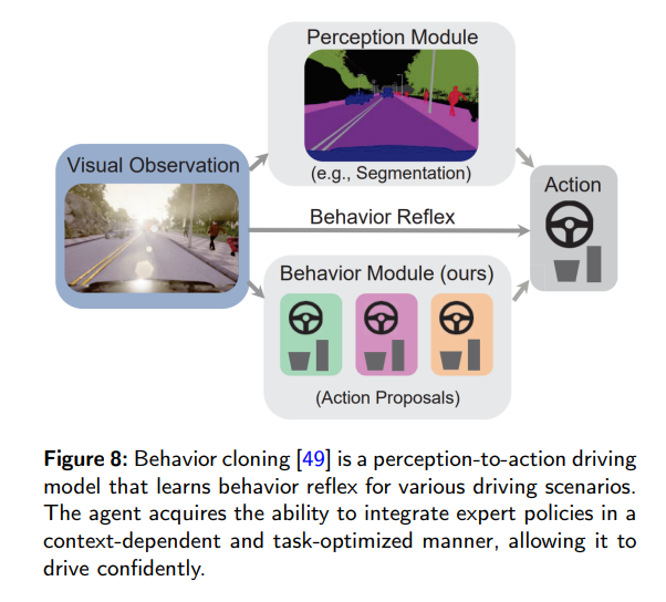
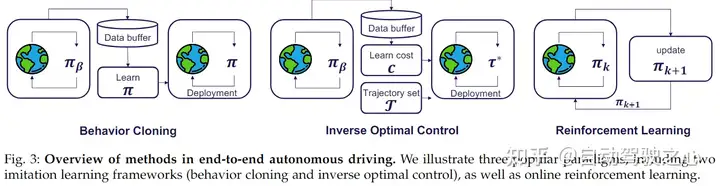
3.2 Behavior Cloning
In behavior cloning, the goal is to match the agent’s policy with the expert’s policy by minimizing planning loss, which is a supervised learning problem on the selected dataset. Behavior cloning has advantages due to its simplicity and efficiency, as it does not require handcrafted reward design, which is critical for reinforcement learning. However, behavior cloning has common issues. During training, behavior cloning treats each state as an independent and identical distribution, leading to a significant issue known as covariate shift. For general IL, several strategy-based methods have been developed to address this issue. In the context of end-to-end autonomous driving, DAgger has been adopted. Another common problem with behavior cloning is causal confusion, where imitators rely on false correlations between certain input components and output signals.
3.3 Reinforcement Learning (RL)
Reinforcement learning is a promising method for addressing distribution shift problems. It aims to maximize cumulative rewards over time through interaction with the environment, with the network making driving decisions based on its actions to gain rewards or penalties. IL cannot handle new situations that significantly differ from the training dataset, while RL is robust when exploring scenarios in a given environment. Reinforcement learning includes various models, such as value-based models like Deep Q-Networks (DQN), Deep Deterministic Policy Gradient (DDPG), and Asynchronous Actor-Critic (A3C).
3.4 Inverse Optimal Control
Traditional IOC algorithms learn the unknown reward function R(s,a) in Markov Decision Processes (MDP) from expert demonstrations, where the expert’s reward function can be represented as a linear combination of features. However, in continuous high-dimensional autonomous driving scenarios, defining rewards is implicit and difficult to optimize.
Generative Adversarial Imitation Learning (GAIL) is a specialized method within IOC that designs the reward function as an adversarial objective to distinguish between expert and learned policies, similar to the concept of Generative Adversarial Networks (GANs). Recently, some work has proposed using auxiliary perception tasks to optimize cost quantities or cost functions. Since costs are an alternative representation of rewards, these methods are classified under the IOC domain. The cost learning framework is defined as follows: end-to-end methods combine other auxiliary tasks to learn reasonable costs c(·) and use simple non-learnable algorithm trajectory samplers to select the trajectory τ* with minimal cost, as shown in Figure 3.
3.5 Online Evaluation (Closed Loop) and Offline Evaluation (Open Loop)
Online Evaluation (Closed Loop):
Testing autonomous driving systems in the real world is costly and risky. To address this challenge, simulation is a viable alternative. Simulators aid in rapid prototyping and testing, enabling quick iterations of ideas and providing low-cost access to a wide range of scenarios. Moreover, simulators offer reliable and accurate tools for measuring performance. However, their primary drawback is that results obtained in simulated environments may not necessarily generalize to the real world.
Offline Evaluation (Open Loop):
Open-loop evaluation involves assessing the system’s performance based on pre-recorded expert driving behavior. This method requires an evaluation dataset that includes (1) sensor readings, (2) target positions, and (3) corresponding future driving trajectories, typically obtained from human drivers. Given the sensor input and target position from the dataset, performance is measured by comparing the system’s predicted future trajectories with those in human driving logs. The system’s evaluation is based on how well its trajectory predictions match human ground truth, along with auxiliary metrics like collision probabilities with other agents. The advantages of open-loop evaluation are its ease of implementation and the absence of a need for simulators, allowing access to real traffic and sensor data. However, a key drawback is that it cannot measure the system’s performance in the actual test distribution encountered during deployment.
3.6 World Models and Model-Based RL
World models are the next milestone in AI following the breakthroughs in NLP (human capabilities). Bengio and LeCun have called for research into world models for five or six years. Undoubtedly, this will be a major goal for academia and industry in the coming years. Prediction is the natural manifestation of world models. By predicting what happens in the next few seconds, one can further understand the changes in the real-world environment.
World Models typically train using self-supervised methods from the environment, with the basic idea being to learn and predict future states through the model itself. Specifically, the training of world models includes the following key components:
-
Perception Model (Vision Model): This part is usually a convolutional neural network responsible for extracting useful features from raw pixel data. This model can predict the content of the next frame by observing consecutive frames, achieving environmental perception, which is somewhat similar to diffusion, with supervision coming from the next frame image.
-
Memory Model: Often employing recurrent neural networks (like LSTM), used to maintain and update the memory state of the environment. This model captures the dynamic changes in the environment by processing time-series data, helping the model better understand the temporal dependencies in the environment, with supervision coming from temporal data.
-
Controller: This part is usually a simple network structure that decides actions based on the outputs of the perception and memory models. The training of the controller may use some reinforcement learning strategies, but it is still optimized based on the self-supervised signals predicted by the model.
In such a setup, the world model trains itself by predicting the future states of the environment (such as the next frame image or the possible state at the next moment). This prediction task itself is a form of self-supervised learning, as it does not require external supervisory signals (like labels or indicators); the model simply trains by predicting the future version of its input data. This allows the world model to evolve itself in complex environments and improve its decision-making process.
In autonomous driving, end-to-end driving can be achieved through either reinforcement learning (RL) to explore and improve the driving model or imitation learning (IL) to train it in a supervised manner to simulate human driving behavior. The supervised learning paradigm aims to learn driving styles from expert demonstrations as training examples for the model.
However, scaling IL-based autonomous driving systems is challenging, as it is impossible to cover every instance during the learning phase. On the other hand, RL’s function is to maximize cumulative rewards over time through interaction with the environment, with the network making driving decisions based on its actions to gain rewards or penalties. Furthermore, RL model training is conducted online, allowing exploration of the environment during training, which is less effective in utilizing data compared to imitation learning. Table 3 summarizes the mainstream methods for end-to-end approaches:

4. Key Points of Self-Supervised Learning
In practical tasks, designing effective auxiliary tasks according to the characteristics of one’s own data is the key to self-supervised learning and its difficulty. When designing self-supervised auxiliary tasks, the following three points need to be considered:
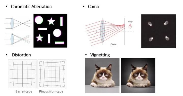
4.1 Shortcuts
Designing auxiliary tasks based on one’s data and task characteristics often yields significant results. For example, for lens detection tasks, obtaining information on imaging color differences, lens distortion, and vignetting to construct auxiliary tasks is quite effective.
4.2 Complexity of Auxiliary Tasks
Previous experimental results have shown that auxiliary tasks are not necessarily more effective when they are more complex. For example, in image reassembly tasks, the optimal number of patches is 9; too many patches lead to insufficient features for each patch and minimal differences between adjacent patches, resulting in poor learning outcomes.
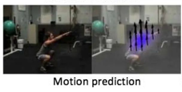
4.3 Ambiguity
Ambiguity means that the labels of the designed auxiliary tasks must be uniquely determined; otherwise, noise will be introduced into the network learning, affecting model performance. For example, in action prediction, the action of a half-squat has ambiguity, as its next state could be either squatting or standing up, making the label non-unique.