▌1. Introduction:
As a beginner in AI, I referenced some articles and wanted to take some notes to deepen my understanding. I am sharing this for those who need it, and I hope it helps others as well!
[Toxic Chicken Soup]: Algorithms often leave you in a state of confusion –> “Who am I, where am I?” No worries, if you keep learning diligently, you will eventually understand, as there are countless algorithms waiting for you.

This article is quite dry, comparable to the Sahara Desert. Even though I picked this article myself, I have to read it through with tears!
▌2. Popular Science:
-
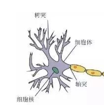
A biological neuron receives stimuli from all directions (inputs) and then reacts (outputs). Just give it a bit of ☀️, and it will shine.
-
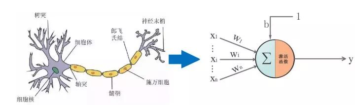
Imitating this, some people proposed artificial neural networks. The foundation of everything –> artificial neural units, see the diagram:
▌3. The Entrance to the Desert: What is a Neuron and What is its Use:
Before starting, it is important to clarify a key question: What is a neuron in artificial neural networks and what is its use? Only by understanding this question can you know where you are, what you are doing, and where you are going.
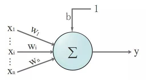
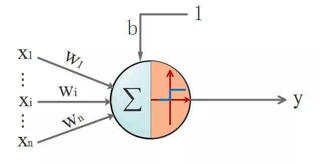
First, let’s review the structure of a neuron. See the diagram below, we will ignore the activation function for now:

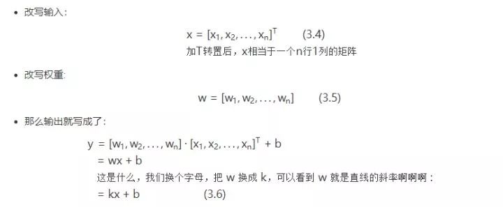
That’s right, we are starting to show formulas! Our data is discrete, and to make it clearer, we will express the discrete data as vectors. You haven’t forgotten what a vector is, have you? You might want to check in with your former PE teacher!
Now, let’s answer the earlier question:
-
What is a neuron: Referring to equation (1.6), from the perspective of the function graph, this is just a straight line.
-
What is a neuron’s use: To explain its use, we need to provide an application scenario: classification. A neuron is just a straight line, equivalent to the boundary between two classes, which can separate red and green pieces. In this case, it acts as a classifier. Therefore, in linear scenarios, a single neuron can achieve classification; it will always learn a suitable straight line to distinguish between the two types of elements.
Take a quick look at the effect diagram, you can play with it yourself: Portal
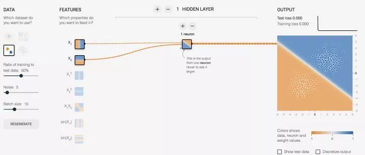
Let me briefly explain the above diagram:
-
(x1,x2) are the inputs to the neuron, and for us, this data represents the coordinates of the points, which we habitually write as (x,y).
We need to make a judgment on the output of the neuron, so we need a judgment rule. By following the judgment rule, we can obtain the results we want. The rule is as follows:
-
Assume, 0 represents a red point, and 1 represents a blue point (these data are pre-labeled, and under supervised learning, the neuron will know the color of the point and use this known result as a benchmark for learning).
-
When the neuron’s output is less than or equal to 0, the final output is 0, which is a red point.
-
When the neuron’s output is greater than 1, the final output is 1, which is a blue point.
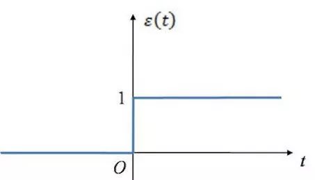
The rules mentioned above remind me of the activation function! (This is just a linear scenario, although it is not suitable, for simplicity, we used the unit step function to describe the function of the activation function.) When x<=0, y = 0; when x > 0, y = 1.
This is the appearance of the step function:
This is the appearance of the neuron:
▌4. The First Step in the Vast Desert: What is an Activation Function and What is its Use
The previous example actually already illustrates the role of the activation function; however, the problems we usually face are not simple linear problems, so we cannot use the unit step function as the activation function, because:
The step function is discontinuous at x=0, meaning it is not differentiable, and its derivative is 0 at non-zero points. In simpler terms, it has outputs limited to [0-1], but it does not have the smooth characteristics that are very important. Moreover, the derivative is 0 at non-zero points, meaning it is hard saturated, and there is simply no gradient, which is also important. The gradient indicates that there is a response in the neuron propagation, rather than being “dead”.
Next, I will explain the characteristics of the activation function, highlighting the important points:
-
Non-linearity: The derivative is not a constant; otherwise, it degenerates into a straight line. For some problems where drawing a straight line still cannot separate them, non-linearity can bend the line, and once it bends, it can encompass everything.
-
Almost everywhere differentiable: This means it has a “smooth characteristic”; don’t overreact, just be normal. Mathematically, being differentiable everywhere provides the core condition for the subsequent backpropagation algorithm (BP algorithm).
-
Limited output range: Generally limited to [0,1], the limited output range makes the neuron relatively stable for larger inputs.
-
Non-saturation: Saturation means that when the input is relatively large, the output changes very little, which can lead to gradient vanishing! What is gradient vanishing: it’s like giving flowers to a girl every day, at first she is surprised, but later she becomes numb and unresponsive. The negative impact of gradient vanishing is that it limits the expressive capability of the neural network; have you ever felt at a loss for words? Sigmoid and tanh functions are soft saturated, while the step function is hard saturated. Soft means that when the input approaches infinity, the output approaches the upper limit, while hard means that for a step function, as long as the input is non-zero, the output is always at the upper limit. I won’t bother with the mathematical representation here; the portal is here (https://www.cnblogs.com/rgvb178/p/6055213.html), which contains detailed explanations. If the activation function is saturated, the defects it brings will slow down the system’s iterative updates, and the system convergence will be slow. Of course, there are ways to compensate for this, one method is to use the cross-entropy function as the loss function; I won’t elaborate on this here. ReLU is non-saturated, and I have personally tested it, and it works pretty well, which is why it has become popular recently.
-
Monotonicity: The sign of the derivative remains unchanged. The derivative is either always greater than 0 or always less than 0, without jumping around. The unchanged sign of the derivative makes it easier for the neural network to converge during training.
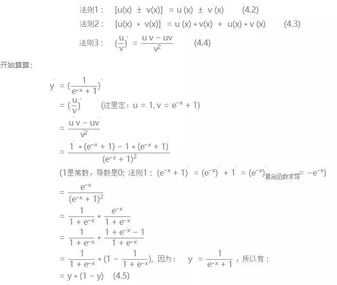
Here, I will only mention the activation functions we use:

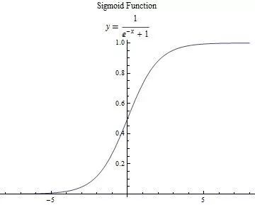
Let’s calculate its derivative, as it will be directly applied in the BP algorithm later:
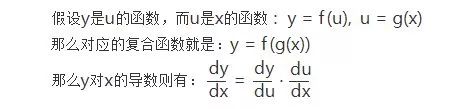
First, let’s invoke the powerful composite function differentiation rule from high school mathematics:
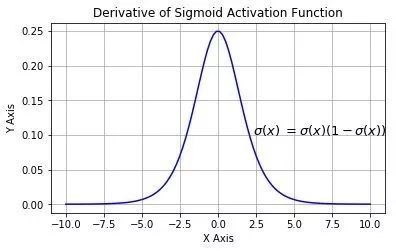
This is the graph of its derivative:
▌5. The Storm in the Center of the Desert: BP (Back Propagation) Algorithm
1. Structure of Neural Networks
After the above introduction, a single neuron is not enough to excite people; only by forming a network can we do so. A neural network is a layered structure, generally consisting of an input layer, hidden layers, and an output layer. Therefore, a neural network has at least 3 layers, with more than 1 hidden layer; if the total number of layers is greater than 3, we refer to it as deep learning.
-
Input Layer: This layer receives raw data and sends it to the hidden layers.
-
Output Layer: The decision output of the neural network.
-
Hidden Layer: This layer is crucial to the neural network, as it performs feature extraction on the data. The significance of the hidden layer is to transform the vector from the previous layer into a new vector. It involves coordinate transformation, which means translating, rotating, scaling, and distorting the data to make it linearly separable. This might be hard to understand, so let’s use an example:
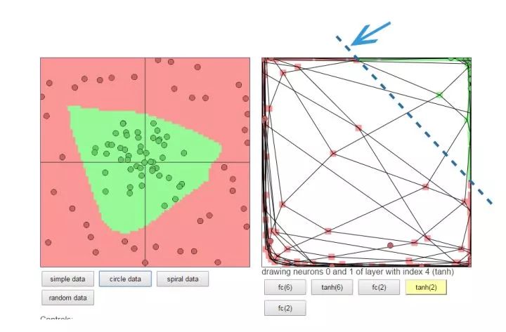
The left diagram shows the original data, with many green points in the middle and many red points on the outskirts. If you were the neural network, what would you do?
One approach: Treat the left diagram as a piece of fabric, sew it into a closed bag (equivalent to transforming the data into a 3D coordinate space), then pull the part with green points to the top (scaling and distorting), and the outer red points will naturally be on the other end. If the position is not cool enough, just shift it a bit (translation). At this point, a clean cut can completely separate the green and red points.
Let me emphasize an important point again: The neural network plays with data in different coordinate spaces. Depending on the needs, it can reduce dimensions, increase dimensions, enlarge, shrink, and flatten; that’s how “invincible” it is.
You can also play with this yourself to intuitively feel it: Portal
2. Forward and Backward Propagation Process
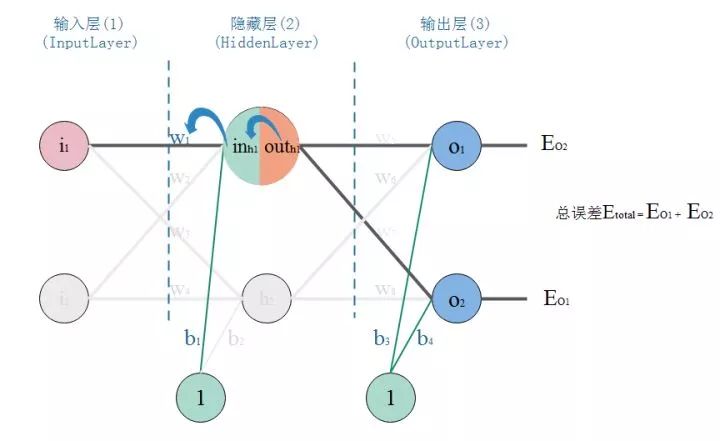
See the diagram, this is a typical three-layer neural network structure. The first layer is the input layer, the second layer is the hidden layer, and the third layer is the output layer. PS: Depending on different application scenarios, the structure of the neural network needs to be designed accordingly. Here, we are only using this simple structure for algorithm derivation and computational convenience.

We will use the scenario of a soldier shooting at a target, where the goal is to train the soldier to hit the target center and become a sharpshooter:
We have some data: the positions (x,y) of a bunch of guns and the shooting results, whether they hit the target or not.
Our goal is to train a neural network model that, given a point’s coordinates (shooting posture), can tell you what the result is (whether it hits the target).
Our method is to train a model that can continuously adjust itself based on errors:
-
Forward Propagation: Input the coordinates of the point into the neural network, and then propagate through each layer until the output layer produces a result.
-
Backward Propagation (BP): It’s like a soldier going to the shooting range. The position of the gun (input) and the target center (expected output) are known. At first, the soldier (neural network) does this randomly, shoots once (the parameters w and b are initialized to random values), observes the result (this is equivalent to performing a forward propagation). Then he realizes he is off to the left of the target center and should aim a bit to the right. So, he adjusts his shooting direction slightly to the right based on the distance from the target center (error, also known as loss). This completes a backward propagation.
-
After one forward and backward propagation, we complete one iteration of neural network training. By repeatedly adjusting the shooting angle (iterating), the error gets smaller and smaller, and the sharpshooter model is born.
3. Derivation and Calculation of BP Algorithm
-
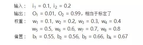
Parameter Initialization:
-
Forward Propagation:
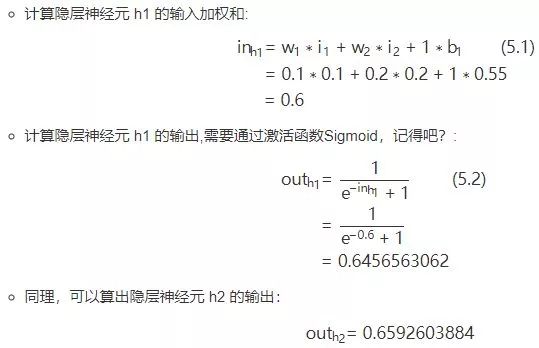
2. From Hidden Layer to Output Layer:
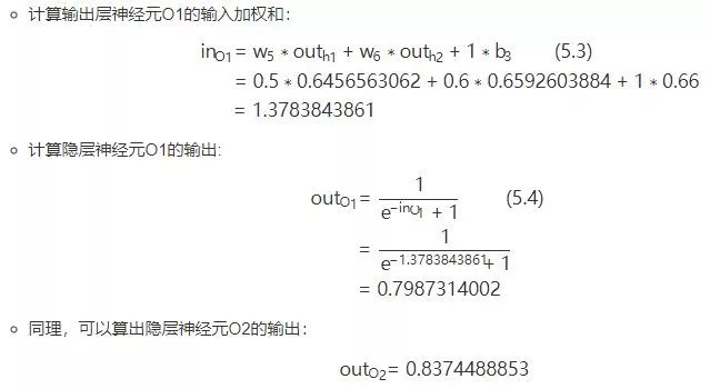
Forward propagation is complete, and we see the output result from the output layer: [0.7987314002, 0.8374488853], but we hope it can output [0.01, 0.99], so the difference is obvious. At this point, we need to use backward propagation to update the weights w and recalculate the output.
-
Backward Propagation:
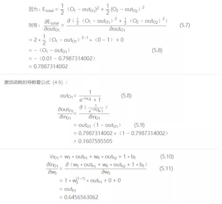
1. Calculate the output error:
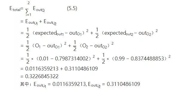
PS: Here I want to mention that this is used as the error calculation because it is simple. In practice, it doesn’t perform very well. If the activation function is saturated, the defects it brings will slow down the system’s iterative updates, and the system convergence will be slow. Of course, there are ways to compensate for this. One method is to use the cross-entropy function as the loss function.
The cross-entropy as the cost function can optimize the convergence of the system because it cancels out the activation function’s derivative term when calculating the gradient of the error with respect to the input, thus avoiding the negative impact brought by the activation function’s “saturation”. If you want to understand more detailed proofs, you can click on the portal (https://blog.csdn.net/lanchunhui/article/details/50086025).

For the output partial derivative:

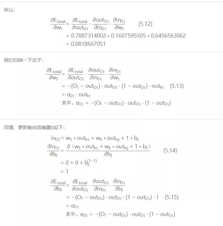
2. Updating weights and biases b from hidden layer to output layer:
-
Let’s first release the chain rule:
-
Taking updating w5 as an example:
We know that the size of weight w directly affects the output. If w is inappropriate, it will cause output errors. To understand how much a certain w value affects the error, we can express it using the rate of change of the error with respect to that w. If a tiny change in w leads to a large increase in error, it means that this w has a greater impact on the error, i.e., the rate of change of the error with respect to that w is higher. The rate of change of the error with respect to w is the partial derivative of the error with respect to w.
So, looking at the diagram, the total error is primarily influenced by the output of the output layer neuron O1, which is then affected by its input, and its input is influenced by w5. This is a chain reaction, finding the root cause from the outcome.
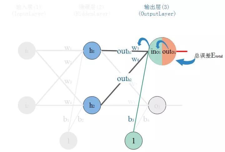
So, according to the chain rule, we have:

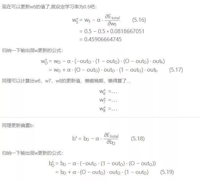
Now, let’s calculate one by one:
There is something called learning rate, let’s set it to 0.5. Regarding the learning rate, it cannot be too high or too low. The training process of the neural network system is about iteratively finding the parameters that minimize the system output error. Each iteration goes through backward propagation to perform gradient descent. However, the error space is not a slide; it’s usually like a bumpy mountain. If the learning rate is too small, it can easily get stuck in a local optimum, meaning the minimum point you think is not the overall minimum point. If the learning rate is too high, the system may struggle to converge, bouncing around and unable to align with the target (the target being the lowest point in the error space). You can see in the diagram:
The x and y axes represent the weight w plane, and the z axis represents the total output error. The entire error surface shows two obvious low points; clearly, the right one is the lowest and represents the global optimum, while the left one is the second lowest and, from a local perspective, is a local optimum. The two paths marked in the diagram represent the ideal gradient descent paths to reach the low points.

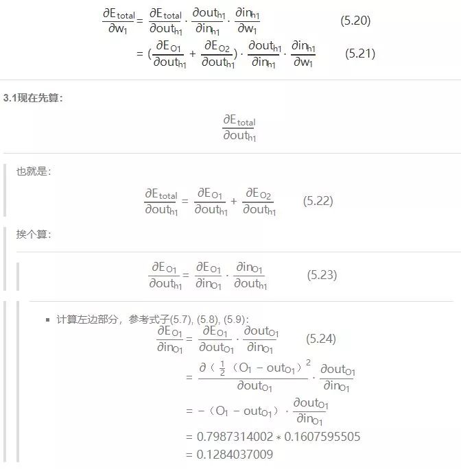
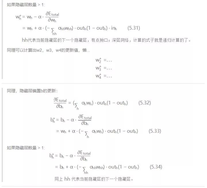
3. Updating weights and biases b from input layer to hidden layer:
-
Taking updating w1 as an example: Upon careful observation, when calculating the update for w5, the error backpropagation path is from the output layer to the hidden layer, i.e., out(O1) to in(O1) to w5. The total error can only be transmitted back through one path. However, when calculating w1, the error backpropagation path is from the hidden layer to the input layer, but there are two paths from the hidden layer neurons. Therefore, when calculating the partial derivative, we need to separate the calculations. See the diagram:
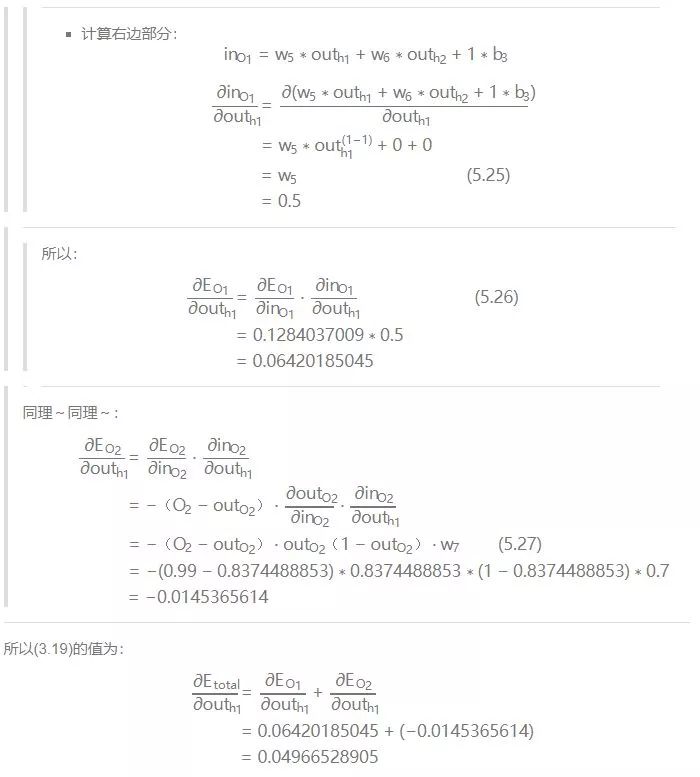
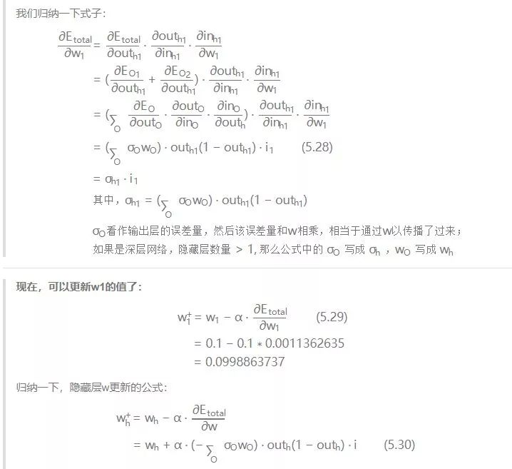
Now, let’s start calculating the total error with respect to w1:

4. Conclusion:
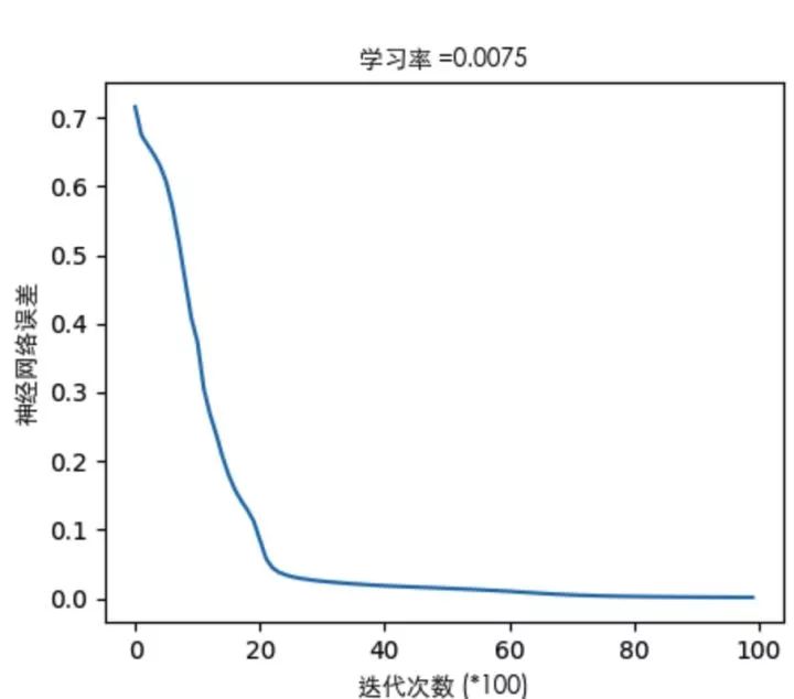
Through hands-on calculations, we have gone through forward propagation and experienced backward propagation, completing one training (iteration). As the iterations deepen, the output layer’s error will become smaller and smaller; in professional terms, the system tends to converge. Here’s a graph showing how system error changes with the number of iterations:

▌6. The Oasis in the Desert: Code Implementation
1. Code Code!
Actually, there are many machine learning frameworks that can easily implement neural networks. However, our goal is: after understanding the algorithm, can we implement the entire process according to the algorithm? This will deepen our understanding of the algorithm’s principles and implementation ideas. By the way, I want to give a shoutout to the numpy library; you deserve it!
-
The code implementation is as follows. The code has been annotated as much as possible, and key implementation points are referenced by formula numbers. If there are parts that are not clear, feel free to revisit the algorithm derivation. The corresponding code has also been uploaded to GitHub.
-
The code allows you to define the structure of the neural network and supports deep networks. It implements a model that classifies red and blue color points through a three-layer network structure, altering the number of neurons in the hidden layer to visually demonstrate the impact of hidden layer neuron count on the problem’s explanatory ability.
-
The code also implements different activation functions. The hidden layer can switch between activation functions as needed, while the output layer generally uses sigmoid, but feel free to change it as you like~
#coding:utf-8
import h5py
import sklearn.datasets
import sklearn.linear_model
import matplotlib
import matplotlib.font_manager as fm
import matplotlib.pyplot as plt
import numpy as np
np.random.seed(1)
font = fm.FontProperties(fname='/System/Library/Fonts/STHeiti Light.ttc')
matplotlib.rcParams['figure.figsize'] = (10.0, 8.0)
def sigmoid(input_sum):
    """
    Function:
        Activation function Sigmoid
    Input:
        input_sum: Input, i.e., the weighted sum of the neuron
    Returns:
        output: Activated output
        input_sum: Return the input for caching
    """
    output = 1.0/(1+np.exp(-input_sum))
    return output, input_sum
def sigmoid_back_propagation(derror_wrt_output, input_sum):
    """
    Function:
        Partial derivative of error with respect to neuron input: dE/dIn = dE/dOut * dOut/dIn  Refer to equation (5.6)
        Where: dOut/dIn is the derivative of the activation function dy=y(1 - y), see equation (5.9)
              dE/dOut is the partial derivative of the error with respect to the neuron output, see equation (5.8)
    Input:
        derror_wrt_output: Partial derivative of error with respect to the neuron output: dE/dyⱼ = 1/2(d(expect_to_output - output)**2/doutput) = -(expect_to_output - output)
        input_sum: Input weighted sum
    Returns:
        derror_wrt_dinputs: Partial derivative of error with respect to input, see equation (5.13)
    """
    output = 1.0/(1 + np.exp(- input_sum))
    doutput_wrt_dinput = output * (1 - output)
    derror_wrt_dinput =  derror_wrt_output * doutput_wrt_dinput
    return derror_wrt_dinput
def relu(input_sum):
    """
        Function:
            Activation function ReLU
        Input:
            input_sum: Input, i.e., the weighted sum of the neuron
        Returns:
            outputs: Activated output
            input_sum: Return the input for caching
    """
    output = np.maximum(0, input_sum)
    return output, input_sum
def relu_back_propagation(derror_wrt_output, input_sum):
    """
        Function:
            Partial derivative of error with respect to neuron input: dE/dIn = dE/dOut * dOut/dIn
            Where: dOut/dIn is the derivative of the activation function
                  dE/dOut is the partial derivative of the error with respect to the neuron output
        Input:
            derror_wrt_output: Partial derivative of error with respect to the neuron output
            input_sum: Input weighted sum
        Returns:
            derror_wrt_dinputs: Partial derivative of error with respect to input
    """
    derror_wrt_dinputs = np.array(derror_wrt_output, copy=True)
    derror_wrt_dinputs[input_sum <= 0] = 0
    return derror_wrt_dinputs
def tanh(input_sum):
    """
    Function:
        Activation function tanh
    Input:
        input_sum: Input, i.e., the weighted sum of the neuron
    Returns:
        output: Activated output
        input_sum: Return the input for caching
    """
    output = np.tanh(input_sum)
    return output, input_sum
def tanh_back_propagation(derror_wrt_output, input_sum):
    """
    Function:
        Partial derivative of error with respect to neuron input: dE/dIn = dE/dOut * dOut/dIn
        Where: dOut/dIn is the derivative of the activation function tanh'(x) = 1 - x²
              dE/dOut is the partial derivative of the error with respect to the neuron output
    Input:
        derror_wrt_output: Partial derivative of error with respect to the neuron output: dE/dyⱼ = 1/2(d(expect_to_output - output)**2/doutput) = -(expect_to_output - output)
        input_sum: Input weighted sum
    Returns:
        derror_wrt_dinputs: Partial derivative of error with respect to input
    """
    output = np.tanh(input_sum)
    doutput_wrt_dinput = 1 - np.power(output, 2)
    derror_wrt_dinput =  derror_wrt_output * doutput_wrt_dinput
    return derror_wrt_dinput
def activated(activation_choose, input):
    """Wrap the forward activation"""
    if activation_choose == "sigmoid":
        return sigmoid(input)
    elif activation_choose == "relu":
        return relu(input)
    elif activation_choose == "tanh":
        return tanh(input)
    return sigmoid(input)
def activated_back_propagation(activation_choose, derror_wrt_output, output):
    """Wrap the backward activation propagation"""
    if activation_choose == "sigmoid":
        return sigmoid_back_propagation(derror_wrt_output, output)
    elif activation_choose == "relu":
        return relu_back_propagation(derror_wrt_output, output)
    elif activation_choose == "tanh":
        return tanh_back_propagation(derror_wrt_output, output)
    return sigmoid_back_propagation(derror_wrt_output, output)
class NeuralNetwork:
    def __init__(self, layers_strcuture, print_cost = False):
        self.layers_strcuture = layers_strcuture
        self.layers_num = len(layers_strcuture)
        # Exclude the input layer from the count of network layers, as other layers are the true neuron layers
        self.param_layers_num = self.layers_num - 1
        self.learning_rate = 0.0618
        self.num_iterations = 2000
        self.x = None
        self.y = None
        self.w = dict()
        self.b = dict()
        self.costs = []
        self.print_cost = print_cost
        self.init_w_and_b()
    def set_learning_rate(self, learning_rate):
        """Set learning rate"""
        self.learning_rate = learning_rate
    def set_num_iterations(self, num_iterations):
        """Set number of iterations"""
        self.num_iterations = num_iterations
    def set_xy(self, input, expected_output):
        """Set the input and expected output of the neural network"""
        self.x = input
        self.y = expected_output
    def init_w_and_b(self):
        """
        Function:
            Initialize all parameters of the neural network
        Input:
            layers_strcuture: The structure of the neural network, for example, [2,4,3,1], a 4-layer structure:
                The 0th layer input layer receives 2 data, the 1st layer hidden layer has 4 neurons, the 2nd layer hidden layer has 3 neurons, and the 3rd layer output layer has 1 neuron
        Returns: An index table of the neural network parameters for locating weights wᵢ  and biases bᵢ, where i is the network layer number
        """
        np.random.seed(3)
        # The weights of the current neuron layer are an n_i x n_(i-1) matrix, where i is the network layer number, n is the number of nodes in layer i
        # For example, for [2,4,3,1], a 4-layer structure: The 0th layer input layer has 2, so the 1st layer hidden layer has 4 neurons
        # Thus, the weights w of the 1st layer is a 4x2 matrix, such as:
        #    w1 = array([ [-0.96927756, -0.59273074],
        #                 [ 0.58227367,  0.45993021],
        #                 [-0.02270222,  0.13577601],
        #                 [-0.07912066, -1.49802751] ])
        # The bias of the current layer is generally set to 0, the bias is a 1xnᵢ matrix, where nᵢ is the number of nodes in layer i, e.g., for the 1st layer with 4 nodes:
        #    b1 = array([ 0.,  0.,  0.,  0.])
        for l in range(1, self.layers_num):
            self.w["w" + str(l)] = np.random.randn(self.layers_strcuture[l], self.layers_strcuture[l-1])/np.sqrt(self.layers_strcuture[l-1])
            self.b["b" + str(l)] = np.zeros((self.layers_strcuture[l], 1))
        return self.w, self.b
    def layer_activation_forward(self, x, w, b, activation_choose):
        """
        Function:
            Forward propagation of the network layer
        Input:
            x: Current network layer input (i.e., output from the previous layer), generally all training data, i.e., the input matrix
            w: Current network layer weight matrix
            b: Current network layer bias matrix
            activation_choose: Choose activation function "sigmoid", "relu", "tanh"
        Returns:
            output: Activated output of the network layer
            cache: Cache the information of the network layer for later use: (x, w, b, input_sum) -> cache
        """
        # Calculate the weighted sum for the input, see equation (5.1)
        input_sum = np.dot(w, x) + b
        # Activate the weighted sum of the input
        output, _ = activated(activation_choose, input_sum)
        return output, (x, w, b, input_sum)
    def forward_propagation(self, x):
        """
        Function:
            Forward propagation of the neural network
        Input:
        Returns:
            output: Output from the forward propagation after completion
            caches: Cache the parameters of each network layer during forward propagation: (x, w, b, input_sum),... -> caches
        """
        caches = []
        # As the input layer, output = input
        output_prev = x
        # The 0th layer is the input layer, which only observes the input data and does not need to process it. Forward propagation starts from the 1st layer until the output layer produces an output.
        # range(1, n) -> [1, 2, ..., n-1]
        L = self.param_layers_num
        for l in range(1, L):
            # The current network layer's input comes from the output of the previous layer
            input_cur = output_prev
            output_prev, cache = self.layer_activation_forward(input_cur, self.w["w"+ str(l)], self.b["b" + str(l)], "tanh")
            caches.append(cache)
        output, cache = self.layer_activation_forward(output_prev, self.w["w" + str(L)], self.b["b" + str(L)], "sigmoid")
        caches.append(cache)
        return output, caches
    def show_caches(self, caches):
        """Display the cached parameter information of the network layers"""
        i = 1
        for cache in caches:
            print("%dth Layer" % i)
            print(" input: %s" % cache[0])
            print(" w: %s" % cache[1])
            print(" b: %s" % cache[2])
            print(" input_sum: %s" % cache[3])
            print("----------")
            i += 1
    def compute_error(self, output):
        """
        Function:
            Calculate the total error of the output after iterations
        Input:
        Returns:
        """
        m = self.y.shape[1]
        # Calculate the error, see equation (5.5): E = Σ1/2(期望输出-实际输出)²
        #error = np.sum(0.5 * (self.y - output) ** 2) / m
        # Cross-entropy as the error function
        error =  -np.sum(np.multiply(np.log(output),self.y) + np.multiply(np.log(1 - output), 1 - self.y)) / m
        error = np.squeeze(error)
        return error
    def layer_activation_backward(self, derror_wrt_output, cache, activation_choose):
        """
            Function:
                Backward propagation of the network layer
            Input:
                derror_wrt_output: Partial derivative of error with respect to output
                cache: Cached information of the network layer (x, w, b, input_sum)
                activation_choose: Choose activation function "sigmoid", "relu", "tanh"
            Returns: Gradient information, i.e.,
                derror_wrt_output_prev: Gradient of error backpropagated to the previous layer's output
                derror_wrt_dw: Gradient of error with respect to weights
                derror_wrt_db: Gradient of error with respect to biases
        """
        input, w, b, input_sum = cache
        output_prev = input     # The output from the previous layer = the input of the current layer; note it is 'input' not the weighted sum of the input (input_sum)
        m = output_prev.shape[1]      # m is the number of samples in the input; we need to take the average, so the following calculations need to be divided by m
        # Implement equation (5.13) -> Partial derivative of error with respect to weights w
        derror_wrt_dinput = activated_back_propagation(activation_choose, derror_wrt_output, input_sum)
        derror_wrt_dw = np.dot(derror_wrt_dinput, output_prev.T) / m
        # Implement equation (5.32) -> Partial derivative of error with respect to biases b
        derror_wrt_db = np.sum(derror_wrt_dinput, axis=1, keepdims=True)/m
        # Provide error transmission for backpropagation to the previous layer, see equation (5.28)'s (Σδ·w) part
        derror_wrt_output_prev = np.dot(w.T, derror_wrt_dinput)
        return derror_wrt_output_prev, derror_wrt_dw, derror_wrt_db
    def back_propagation(self, output, caches):
        """
        Function:
            Backward propagation of the neural network
        Input:
            output: Output from the neural network
            caches: Cached parameter information of all network layers (excluding input layer)  [(x, w, b, input_sum), ...]
        Returns:
            grads: Returns the current iteration's gradient information
        """
        grads = {}
        L = self.param_layers_num #
        output = output.reshape(output.shape)  # Reshape the output layer's output to match the expected output structure
        expected_output = self.y
        # See equation (5.8)
        #derror_wrt_output = -(expected_output - output)
        # Cross-entropy as the error function
        derror_wrt_output = - (np.divide(expected_output, output) - np.divide(1 - expected_output, 1 - output))
        # Backward propagation: Output layer -> Hidden layer, obtaining gradients: see equations (5.8), (5.13), (5.15)
        current_cache = caches[L - 1] # Take the last layer, i.e., the output layer's parameter information
        grads["derror_wrt_output" + str(L)], grads["derror_wrt_dw" + str(L)], grads["derror_wrt_db" + str(L)] = \
            self.layer_activation_backward(derror_wrt_output, current_cache, "sigmoid")
        # Backward propagation: Hidden layer -> Hidden layer, obtaining gradients: see equations (5.28)'s (Σδ·w), (5.28), (5.32)
        for l in reversed(range(L - 1)):
            current_cache = caches[l]
            derror_wrt_output_prev_temp, derror_wrt_dw_temp, derror_wrt_db_temp = \
                self.layer_activation_backward(grads["derror_wrt_output" + str(l + 2)], current_cache, "tanh")
            grads["derror_wrt_output" + str(l + 1)] = derror_wrt_output_prev_temp
            grads["derror_wrt_dw" + str(l + 1)] = derror_wrt_dw_temp
            grads["derror_wrt_db" + str(l + 1)] = derror_wrt_db_temp
        return grads
    def update_w_and_b(self, grads):
        """
        Function:
            Update w and b based on gradient information
        Input:
            grads: Current iteration's gradient information
        Returns:
        """
        # Update weights w and biases b, see equations: (5.16),(5.18)
        for l in range(self.param_layers_num):
            self.w["w" + str(l + 1)] = self.w["w" + str(l + 1)] - self.learning_rate * grads["derror_wrt_dw" + str(l + 1)]
            self.b["b" + str(l + 1)] = self.b["b" + str(l + 1)] - self.learning_rate * grads["derror_wrt_db" + str(l + 1)]
    def training_modle(self):
        """Train the neural network model"""
        np.random.seed(5)
        for i in range(0, self.num_iterations):
            # Forward propagation, obtaining network output and parameters for each layer
            output, caches = self.forward_propagation(self.x)
            # Calculate the network output error
            cost = self.compute_error(output)
            # Backward propagation, obtaining gradient information
            grads = self.back_propagation(output, caches)
            # Update weights w and biases b based on gradient information
            self.update_w_and_b(grads)
            # At the end of this iteration, print error information
            if self.print_cost and i % 1000 == 0:
                print ("Cost after iteration %i: %f" % (i, cost))
            if self.print_cost and i % 1000 == 0:
                self.costs.append(cost)
        # After the model training is complete, display the error curve
        if False:
            plt.plot(np.squeeze(self.costs))
            plt.ylabel(u'Neural Network Error', fontproperties = font)
            plt.xlabel(u'Number of Iterations (*100)', fontproperties = font)
            plt.title(u"Learning Rate =" + str(self.learning_rate), fontproperties = font)
            plt.show()
        return self.w, self.b
    def predict_by_modle(self, x):
        """Use the trained model (i.e., the final w and b parameters obtained) to decide the result of the input sample"""
        output, _ = self.forward_propagation(x.T)
        output = output.T
        result = output / np.sum(output, axis=1, keepdims=True)
        return np.argmax(result, axis=1)
def plot_decision_boundary(xy, colors, pred_func):
    # xy is the collection of coordinate points, calculate the range of the collection
    # Adding and subtracting 0.5 expands the canvas range; otherwise, the plotted points will fall on the edge of the graph, which is a nightmare for perfectionists
    x_min, x_max = xy[:, 0].min() - 0.5, xy[:, 0].max() + 0.5
    y_min, y_max = xy[:, 1].min() - 0.5, xy[:, 1].max() + 0.5
    # Generate a grid of sampling points with resolution h, like a net covering all color points
    h = .01
    xx, yy = np.meshgrid(np.arange(x_min, x_max, h), np.arange(y_min, y_max, h))
    # Use the grid points as input to the model, predicting what color each sampling point is, thus obtaining a decision boundary
    Z = pred_func(np.c_[xx.ravel(), yy.ravel()])
    Z = Z.reshape(xx.shape)
    # Use contour lines to plot the predicted results, effectively drawing the boundary line between red and blue points
    plt.contourf(xx, yy, Z, cmap=plt.cm.Spectral)
    # Also plot the training red and blue points
    plt.scatter(xy[:, 0], xy[:, 1], c=colors, marker='o', cmap=plt.cm.Spectral, edgecolors='black')
if __name__ == "__main__":
    plt.figure(figsize=(16, 32))
    # Use sklearn's data sample set to produce coordinates of two colors, noise is the noise coefficient; the larger the noise, the more chaotic the distribution of the two colors
    xy, colors = sklearn.datasets.make_moons(60, noise=1.0)
    # Since the point colors are 1bit, we design a neural network with 2 output neurons.
    # Label output [1,0] for red points, output [0,1] for blue points
    expect_output = []
    for c in colors:
        if c == 1:
            expect_output.append([0,1])
        else:
            expect_output.append([1,0])
    expect_output = np.array(expect_output).T
    # Design a 3-layer network, changing the number of neurons in the hidden layer to observe the effect of the neural network on classifying red and blue points
    hidden_layer_neuron_num_list = [1,2,4,10,20,50]
    for i, hidden_layer_neuron_num in enumerate(hidden_layer_neuron_num_list):
        plt.subplot(5, 2, i + 1)
        plt.title(u'Number of Neurons in Hidden Layer: %d' % hidden_layer_neuron_num, fontproperties = font)
        nn = NeuralNetwork([2, hidden_layer_neuron_num, 2], True)
        # Both the input and output layers have 2 nodes, so the input and output data sets must be nx2 matrices
        nn.set_xy(xy.T, expect_output)
        nn.set_num_iterations(30000)
        nn.set_learning_rate(0.1)
        w, b = nn.training_modle()
        plot_decision_boundary(xy, colors, nn.predict_by_modle)
    plt.show()
2. Show the Graph!
Regarding the error curve (here’s just one example):
-
By observing the error curve, you can determine the network’s performance to some extent, whether the model training can converge, and the degree of convergence can all be inferred from the error curve during the gradient descent process.
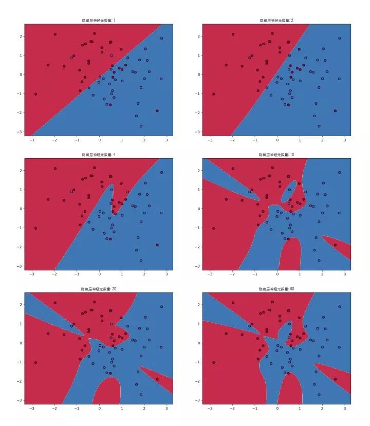
Under the structure of a 3-layer network, with only one hidden layer, let’s explain how the change in the number of hidden layer neurons affects the expressive capability of the neural network:
-
When there is only 1 neuron in the hidden layer: As mentioned at the beginning of the article, a single neuron is just a linear classifier, and its expressive capability is merely a straight line, see equation (3.6).
-
With 2 neurons: The line starts to bend a bit, but the result is still not obvious, awkward. However, from a theoretical perspective, the neural network begins to possess non-linear expressive capability.
-
As the number of neurons in the hidden layer increases, the expressive capability of the neural network strengthens, and the classification effect improves. However, it’s not necessarily the case that more neurons are better; we should start considering whether deeper networks yield better results.
▌7. No Conclusion
Remember one thing, the BP neural network is the simplest among various neural networks. Only by mastering it can you build a foundation for learning other more complex neural networks.
Although we have derived and implemented the algorithm, there are still many questions. This is just to spark some thoughts:
-
What is the most effective structure for a neural network, i.e., how many layers, and how should the input and output be designed?
-
Mathematical theory proves that a three-layer neural network can approximate any nonlinear continuous function to any precision. So why do we need deep networks?
-
How should we choose activation functions in different application scenarios?
-
How should we choose the learning rate?
-
How many training iterations yield the best model performance?
AI, from introduction to giving up, the first article ends.
This article is from Tencent’s Zhihu column:
For more information, please scan the QR code below and follow the Machine Learning Research Association.

Reprinted from: AI Headlines