Advanced PyTorch: Training Deep Neural Networks on GPU

This article is the fourth in this series and will introduce how to train deep neural networks using PyTorch on a GPU.

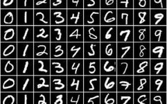
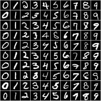
In previous tutorials, we trained a logistic regression model to recognize handwritten digits based on the MNIST dataset, achieving about 86% accuracy.

However, we also noticed that due to the limited capacity of the model, it is difficult to further improve accuracy beyond 87%. In this article, we will attempt to improve accuracy using a feedforward neural network. Most of the content of this tutorial is inspired by Jeremy Howard’s FastAI development notes: https://github.com/fastai/fastai_old/tree/master/dev_nb

If you want to read while running the code, you can find the Jupyter Notebook for this tutorial at the following link:

https://jvn.io/aakashns/fdaae0bf32cf4917a931ac415a5c31b0

You can clone this notebook, install the necessary dependencies using conda, and then start Jupyter by running the following commands in the terminal:

pip install jovian --upgrade    # Install the jovian library 
jovian clone fdaae0bf32cf4917a931ac415a5c31b0  # Download notebook
cd 04-feedforward-nn            # Enter the created directory 
jovian install                  # Install the dependencies
conda activate 04-feedforward-nn # Activate virtual env
jupyter notebook                # Start Jupyter

If your conda version is older, you may need to run source activate 04-feedforward-nn to activate the virtual environment. For a more detailed explanation of the above steps, refer to the first article in this series of tutorials.

The data preparation process here is exactly the same as in the previous tutorial. We first import the necessary modules and classes.

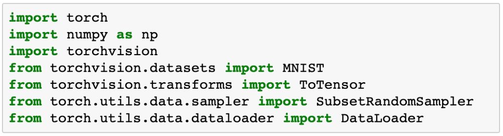
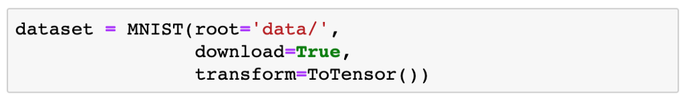
We use the MNIST class from torchvision.datasets to download the data and create a PyTorch dataset.

Next, we define and use a function split_indices to randomly select 20% of the images as the validation set.

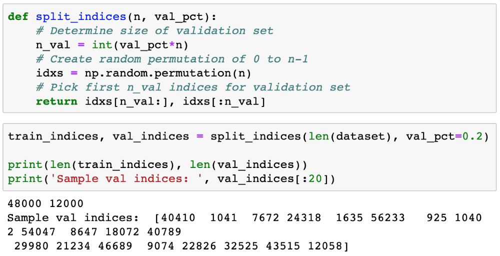
Now, we can use SubsetRandomSampler to create a PyTorch data loader for each subset, which samples elements randomly from a given index list while creating batches of data.

To achieve further improvement based on logistic regression, we will create a neural network with one hidden layer. Here’s our approach:

• We will no longer use a single nn.Linear object to convert the input batch (pixel intensities) into the output batch (class probabilities), but will use two nn.Linear objects. Each of these objects is referred to as a layer, and the model itself is called a network.

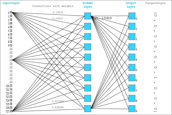
• The first layer (also known as the hidden layer) can convert an input matrix of size batch_size x 784 into an intermediate output matrix of size batch_size x hidden_size, where hidden_size is a preconfigured parameter (e.g., 32 or 64).

• Then, this intermediate output will be passed to a nonlinear activation function that operates on the individual elements of this output matrix.

• The result of this activation function will also be of size batch_size x hidden_size and will be passed to the second layer (also known as the output layer). This layer can convert the hidden layer’s results into a matrix of size batch_size x 10, which is the same as the output of the logistic regression model.

Introducing a hidden layer and an activation function allows the model to learn more complex, multi-layered, and nonlinear relationships between inputs and targets. It looks like this (the blue box represents the layer output for a single input image):

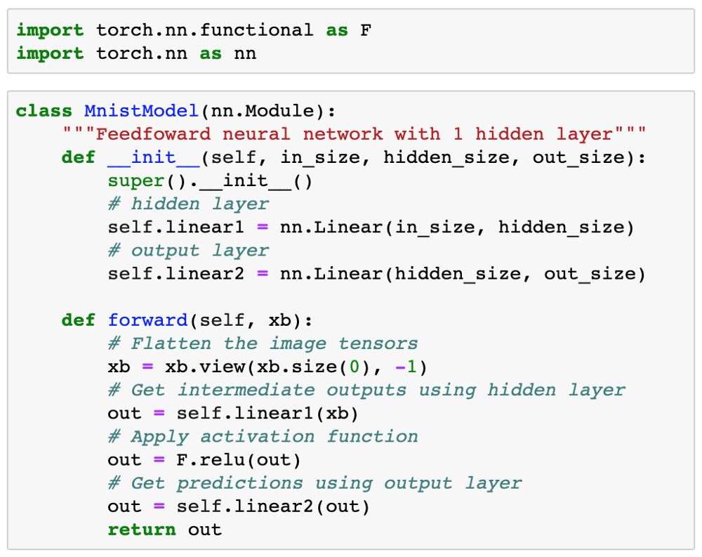
The activation function we will use here is the Rectified Linear Unit (ReLU), which has a simple formula: relu(x) = max(0, x), meaning if an element is negative, it is replaced with 0; otherwise, it remains unchanged.

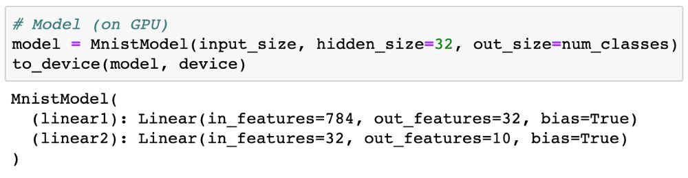
To define the model, we extend the nn.Module class, just as we did with logistic regression.

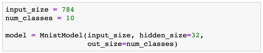
We will create a model with a hidden layer of 32 activations.

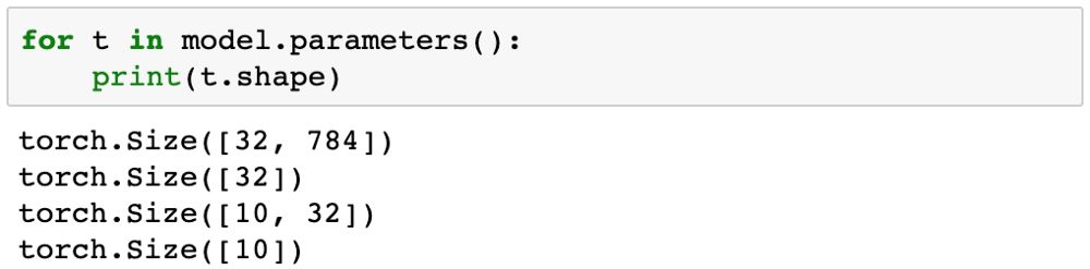
Let’s take a look at the model parameters. It is expected that each layer has a weight and bias matrix.

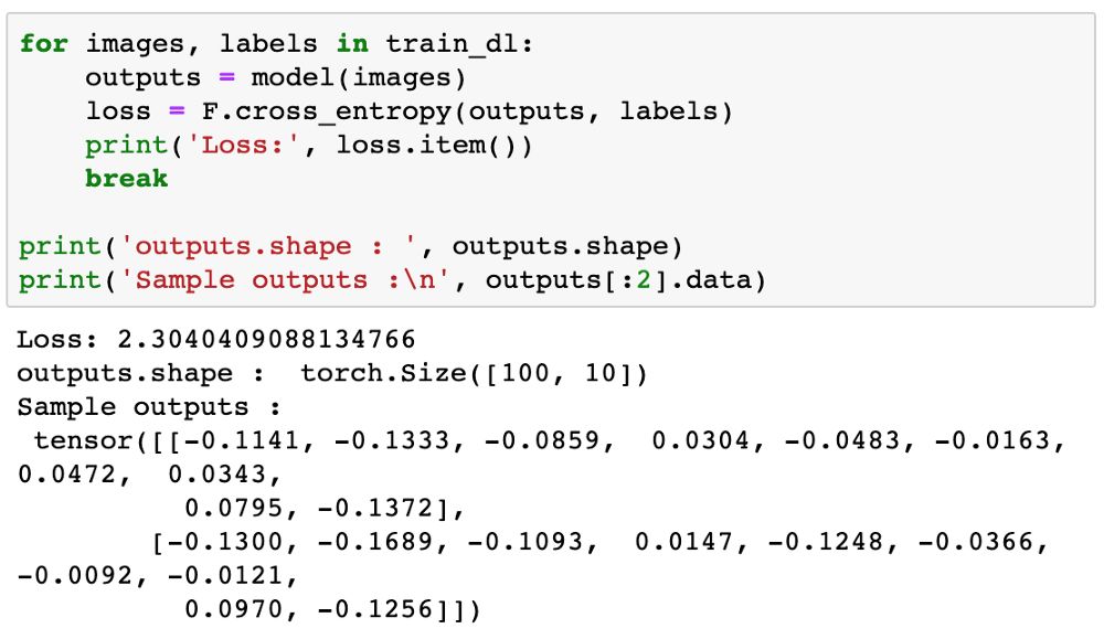
Let’s try to generate some outputs using our model. We take the first batch of 100 images from our dataset and feed them into our model.

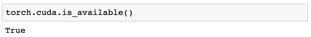
As our model and dataset size increase, we need to use a GPU (graphics processing unit, also known as a video card) to train our model in a reasonable time. The GPU contains hundreds of cores optimized for costly floating-point matrix operations, allowing us to complete these calculations in a shorter time; this makes the GPU very suitable for training deep neural networks with many layers. You can use GPUs for free on Kaggle kernels or Google Colab, or rent GPU usage services from Google Cloud Platform, Amazon Web Services, or Paperspace. You can check if the GPU is available and if the necessary NVIDIA drivers and CUDA libraries are installed using torch.cuda.is_available.

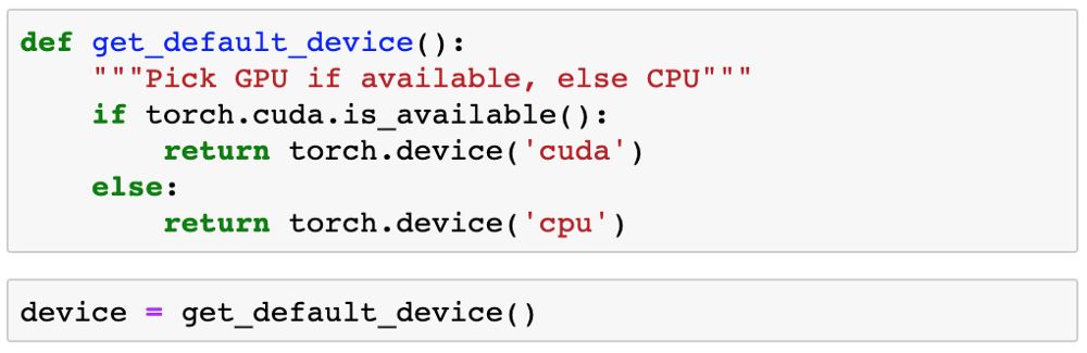
We define a helper function to select the GPU as the target device when available, otherwise default to CPU.

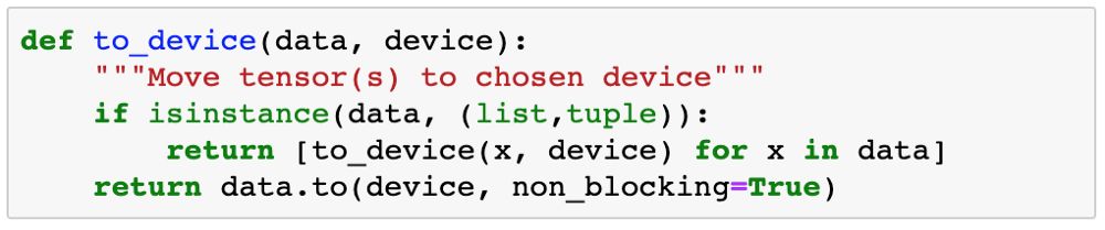
Next, we define a function to move data to the selected device.

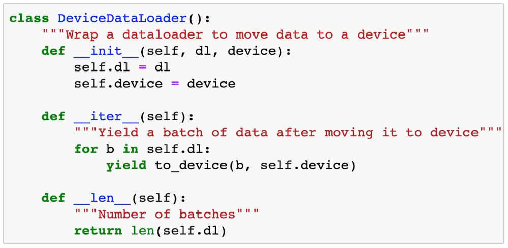
Finally, we define a DeviceDataLoader class (inspired by FastAI) to encapsulate our existing data loaders and move the data to the selected device when reading data batches. Interestingly, we do not need to extend existing classes to create PyTorch data loaders. We only need to use the __iter__ method to retrieve data batches and the __len__ method to get the number of batches.

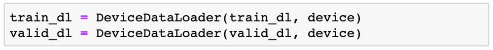
We can now use DeviceDataLoader to encapsulate our data loaders.

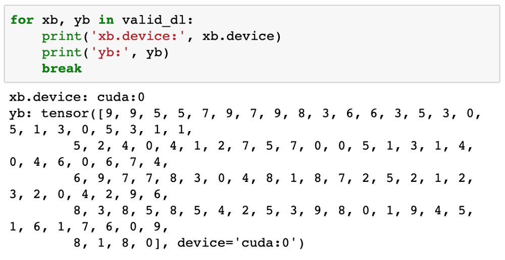
The tensors moved to the GPU’s RAM have a device attribute that contains the word cuda. We can verify this by looking at a batch of data from valid_dl.

Similar to logistic regression, we can use cross-entropy as the loss function and accuracy as the evaluation metric for the model. The training loop is also the same, so we can reuse the loss_batch, evaluate, and fit functions from the previous tutorial.

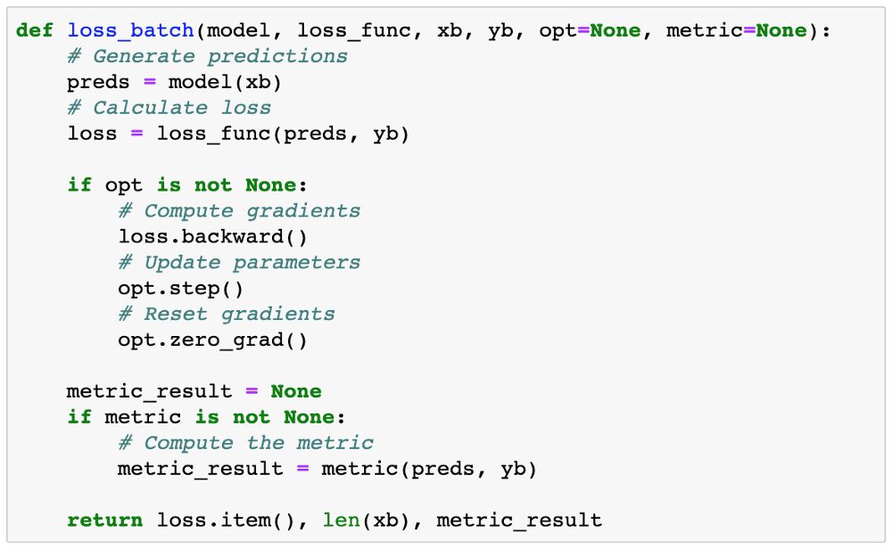
The loss_batch function computes the loss and metric values for a batch of data, and can optionally perform gradient descent if an optimizer is provided.

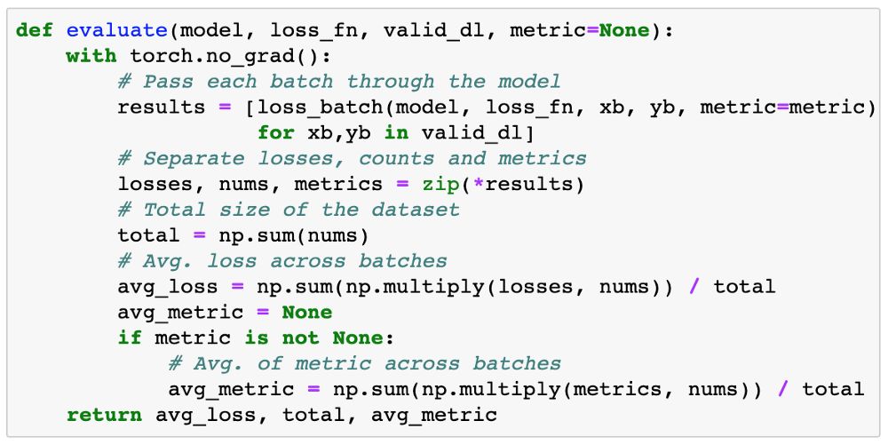
The evaluate function computes the overall loss for the validation set (and a metric if available).

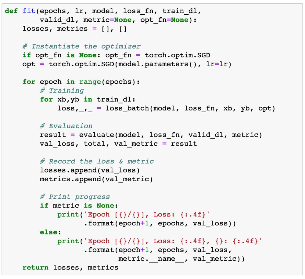
Like the definitions in the previous tutorial, the fit function contains the actual training loop. We will make some improvements to the fit function:

• We do not manually define the optimizer; instead, we pass in the learning rate and create an optimizer within the function. This allows us to train the model with different learning rates when needed.

• We will log the validation loss and accuracy at the end of each epoch and return this history as the output of the fit function.

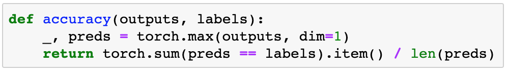
We also need to define an accuracy function that calculates the overall accuracy of the model on a batch of outputs, so we can use it as a metric in fit.

Before we train the model, we need to ensure that the data and model parameters (weights and biases) are on the same device (CPU or GPU). We can reuse the to_device function to move the model parameters to the correct device.

Let’s see how the model performs on the validation set using the initial weights and biases.

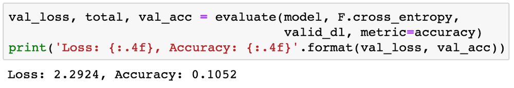
The initial accuracy is about 10%, which is consistent with our expectations for a randomly initialized model (which has a one in ten chance of getting the correct label).

Now we can start training the model. We will first train for 5 epochs to see the results. We can use a relatively high learning rate of 0.5.

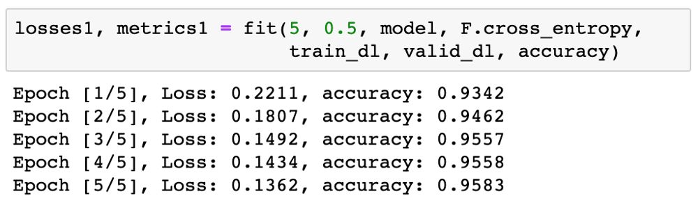
95% is very good! We will further train for 5 epochs with a lower learning rate of 0.1 to improve accuracy.

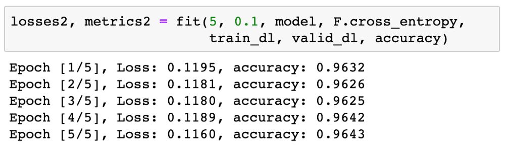
Now we can plot the accuracy chart to see how the model improves over time.

Our current model greatly outperforms the logistic model (which could only achieve about 86% accuracy)! It quickly reached 96% accuracy but failed to improve further. To enhance accuracy further, we need to make the model more powerful. You might have guessed it, increasing the size of the hidden layer or adding more hidden layers can achieve this.

Finally, we can use the jovian library to save and submit our results.

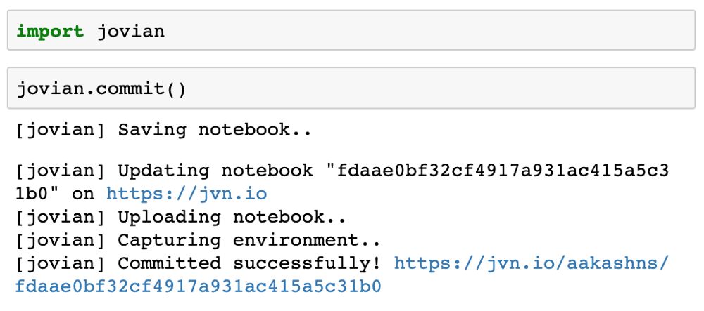
Jovian will upload the notebook to https://jvn.io, retrieve its Python environment, and create a shareable link for the notebook. You can use this link to share your results, allowing anyone to easily reproduce it using the jovian clone command. Jovian also has a powerful commenting interface that allows you and others to discuss and comment on various parts of your notebook.

The topics covered in this tutorial are summarized as follows:

• We created a neural network with one hidden layer to achieve further improvement based on the logistic regression model from the previous tutorial.

• We used the ReLU activation function to introduce non-linearity, allowing the model to learn more complex relationships between inputs and outputs.

• We defined some utilities like get_default_device, to_device, and DeviceDataLoader to utilize the GPU when available and move input data and model parameters to the appropriate device.

• We can use the same training loop that we defined earlier: the fit function, to train our model and evaluate it on the validation dataset.

There are many areas to experiment with, and I suggest you take advantage of Jupyter’s interactive nature to try various parameters. Here are some ideas:

• Try modifying the size of the hidden layer or adding more hidden layers to see if you can achieve higher accuracy.

• Try modifying the batch size and learning rate to see if you can achieve the same accuracy with fewer epochs.

• Compare training times on CPU and GPU. Do you see a significant difference? How do the dataset size and model size (number of weights and parameters) affect this?

• Try building models for different datasets, such as CIFAR10 or CIFAR100.

Finally, here are some good resources for further learning:

• A visual proof that neural networks can compute any function, also known as the universal approximation theorem: http://neuralnetworksanddeeplearning.com/chap4.html

• What exactly is a neural network? – A visual and intuitive introduction explaining neural networks and what the intermediate layers represent: https://www.youtube.com/watch?v=aircAruvnKk

• Stanford CS229 lecture notes on backpropagation – A more mathematical explanation of how multi-layer neural networks compute gradients and update weights: http://cs229.stanford.edu/notes/cs229-notes-backprop.pdf

• Andrew Ng’s Coursera course: Video lecture on activation functions: https://www.coursera.org/lecture/neural-networks-deep-learning/activation-functions-4dDC1

Good news!
Beginner Learning Visuals Knowledge Circle
is now open to the public 👇👇👇








Download 1: OpenCV-Contrib Extension Module Chinese Version Tutorial
Reply "Extension Module Chinese Tutorial" in the "Beginner Learning Visuals" WeChat public account backend to download the first Chinese version of the OpenCV extension module tutorial available online, covering installation of extension modules, SFM algorithms, stereo vision, object tracking, biological vision, super-resolution processing, and more than twenty chapters.

Download 2: Python Visual Practical Project 52 Lectures
Reply "Python Visual Practical Project" in the "Beginner Learning Visuals" WeChat public account backend to download 31 visual practical projects including image segmentation, mask detection, lane line detection, vehicle counting, eyeliner addition, license plate recognition, character recognition, emotion detection, text content extraction, and face recognition, helping to quickly learn computer vision.

Download 3: OpenCV Practical Project 20 Lectures
Reply "OpenCV Practical Project 20 Lectures" in the "Beginner Learning Visuals" WeChat public account backend to download 20 practical projects based on OpenCV, achieving advanced learning of OpenCV.

Group Chat

Welcome to join the public account reader group to communicate with peers. Currently, we have WeChat groups for SLAM, 3D vision, sensors, autonomous driving, computational photography, detection, segmentation, recognition, medical imaging, GAN, algorithm competitions, etc. (will be gradually subdivided later). Please scan the WeChat ID below to join the group, and mark: "Nickname + School/Company + Research Direction", for example: "Zhang San + Shanghai Jiao Tong University + Visual SLAM". Please follow the format for the remarks, otherwise, they will not be approved. After successful addition, you will be invited to join relevant WeChat groups based on research direction. Please do not send advertisements in the group, otherwise, you will be removed from the group, thank you for your understanding.