
Introduction
Translated by: Lin Buqing(https://www.zhihu.com/people/lu-guo-92-42-88)
https://github.com/fengdu78/machine_learning_beginner/tree/master/PyTorch_beginner
Table of Contents
(1) Tensors
%matplotlib inline
import torch
import numpy as np
Initializing Tensors
Creating Directly from Data
data = [[1, 2],[3, 4]]
x_data = torch.tensor(data)
Creating from Numpy
np_array = np.array(data)
x_np = torch.from_numpy(np_array)
Creating from Other Tensors
x_ones = torch.ones_like(x_data)  # retains the properties of x_data
print(f"Ones Tensor: \n {x_ones} \n")
x_rand = torch.rand_like(x_data, dtype=torch.float)  # overrides the datatype of x_data
print(f"Random Tensor: \n {x_rand} \n")
Ones Tensor:  tensor([[1, 1],        [1, 1]])
Random Tensor: tensor([[0.6075, 0.4581], [0.5631, 0.1357]])shape = (2,3,)
rand_tensor = torch.rand(shape)
ones_tensor = torch.ones(shape)
zeros_tensor = torch.zeros(shape)
print(f"Random Tensor: \n {rand_tensor} \n")
print(f"Ones Tensor: \n {ones_tensor} \n")
print(f"Zeros Tensor: \n {zeros_tensor}")
Random Tensor: tensor([[0.7488, 0.0891, 0.8417], [0.0783, 0.5984, 0.5709]])
Ones Tensor: tensor([[1., 1., 1.], [1., 1., 1.]])
Zeros Tensor: tensor([[0., 0., 0.], [0., 0., 0.]])Properties of Tensors
tensor = torch.rand(3,4)
print(f"Shape of tensor: {tensor.shape}")
print(f"Datatype of tensor: {tensor.dtype}")
print(f"Device tensor is stored on: {tensor.device}")
Shape of tensor: torch.Size([3, 4])
Datatype of tensor: torch.float32
Device tensor is stored on: cpu
Operations on Tensors
# We move our tensor to the GPU if available
if torch.cuda.is_available(): tensor = tensor.to('cuda')Standard Numpy-like Indexing and Slicing:
tensor = torch.ones(4, 4)
tensor[:,1] = 0
print(tensor)
tensor([[1., 0., 1., 1.],        [1., 0., 1., 1.],        [1., 0., 1., 1.],        [1., 0., 1., 1.]])
Concatenating Tensors
t1 = torch.cat([tensor, tensor, tensor], dim=1)
print(t1)
tensor([[1., 0., 1., 1., 1., 0., 1., 1., 1., 0., 1., 1.],        [1., 0., 1., 1., 1., 0., 1., 1., 1., 0., 1., 1.],        [1., 0., 1., 1., 1., 0., 1., 1., 1., 0., 1., 1.],        [1., 0., 1., 1., 1., 0., 1., 1., 1., 0., 1., 1.]])
Adding Tensors
# This computes the element-wise product
print(f"tensor.mul(tensor) \n {tensor.mul(tensor)} \n")
# Alternative syntax:
print(f"tensor * tensor \n {tensor * tensor}")
tensor.mul(tensor)  tensor([[1., 0., 1., 1.],        [1., 0., 1., 1.],        [1., 0., 1., 1.],        [1., 0., 1., 1.]])
tensor * tensor tensor([[1., 0., 1., 1.], [1., 0., 1., 1.], [1., 0., 1., 1.], [1., 0., 1., 1.]])print(f"tensor.matmul(tensor.T) \n {tensor.matmul(tensor.T)} \n")
# Alternative syntax:
print(f"tensor @ tensor.T \n {tensor @ tensor.T}")
tensor.matmul(tensor.T) tensor([[3., 3., 3., 3.], [3., 3., 3., 3.], [3., 3., 3., 3.], [3., 3., 3., 3.]])
tensor @ tensor.T tensor([[3., 3., 3., 3.], [3., 3., 3., 3.], [3., 3., 3., 3.], [3., 3., 3., 3.]])In-Place Operations
print(tensor, "\n")
tensor.add_(5)
print(tensor)
tensor([[1., 0., 1., 1.],        [1., 0., 1., 1.],        [1., 0., 1., 1.],        [1., 0., 1., 1.]])
tensor([[6., 5., 6., 6.],        [6., 5., 6., 6.],        [6., 5., 6., 6.],        [6., 5., 6., 6.]])
Note
Converting Tensors to NumPy Arrays
t = torch.ones(5)
print(f"t: {t}")
n = t.numpy()
print(f"n: {n}")
t: tensor([1., 1., 1., 1., 1.])
n: [1. 1. 1. 1. 1.]
t.add_(1)
print(f"t: {t}")
print(f"n: {n}")
t: tensor([2., 2., 2., 2., 2.])
n: [2. 2. 2. 2. 2.]
Converting NumPy Arrays to Tensors
n = np.ones(5)
t = torch.from_numpy(n)
np.add(n, 1, out=n)(2) Autograd: Automatic Differentiation
torch.autograd is the automatic differentiation tool in PyTorch and is at the core of all neural networks. First, let’s briefly understand how this package trains neural networks.
[3Blue1Brown]:
https://www.youtube.com/watch?v=tIeHLnjs5U8
%matplotlib inline
import torch, torchvision
model = torchvision.models.resnet18(pretrained=True)
data = torch.rand(1, 3, 64, 64)
labels = torch.rand(1, 1000)
prediction = model(data) # Forward propagation
loss = (prediction - labels).sum()
loss.backward()  # Backward propagation
optim = torch.optim.SGD(model.parameters(), lr=1e-2, momentum=0.9)
optim.step() # Gradient descent
import torch
a = torch.tensor([2., 3.], requires_grad=True)
b = torch.tensor([6., 4.], requires_grad=True)
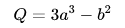
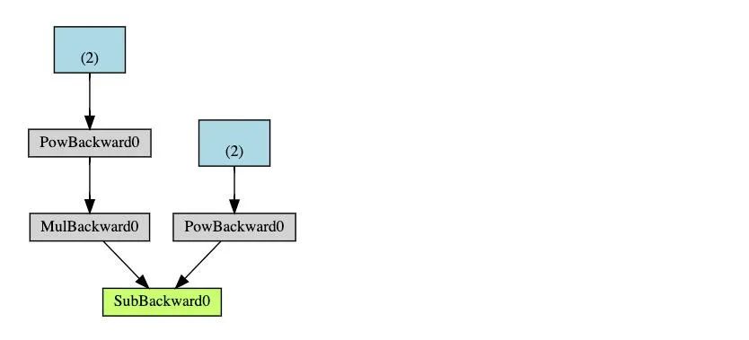
Q = 3*a**3 - b**2

external_grad = torch.tensor([1., 1.])
Q.backward(gradient=external_grad)
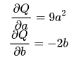
# Check if the stored gradients are correct
print(9*a**2 == a.grad)
print(-2*b == b.grad)
 Then, according to the chain rule, the Jacobian-vector product will be the gradient of 𝑙 with respect to 𝑥⃗.
 .
.-
Runs the requested operations to compute the resulting tensor -
Keeps track of the gradients of operations in the DAG
-
Calculating the gradients of each .grad_fn -
Accumulating them into the .grad attribute of each respective tensor -
Using the chain rule to propagate all the way back to the leaf nodes
Note
x = torch.rand(5, 5)
y = torch.rand(5, 5)
z = torch.rand((5, 5), requires_grad=True)
a = x + y
print(f"Does `a` require gradients? : {a.requires_grad}")
b = x + z
print(f"Does `b` require gradients?: {b.requires_grad}")
from torch import nn, optim
model = torchvision.models.resnet18(pretrained=True)
# Freeze all parameters in the network
for param in model.parameters():    param.requires_grad = False
model.fc = nn.Linear(512, 10)
# Only optimize the classifier
optimizer = optim.SGD(model.fc.parameters(), lr=1e-2, momentum=0.9)
-
[In-place Modification Operations and Multithreaded Autograd]: (https://pytorch.org/docs/stable/notes/autograd.html) -
[Examples of Backward Mode Autodiff]: (https://colab.research.google.com/drive/1VpeE6UvEPRz9HmsHh1KS0XxXjYu533EC)
(3) Neural Networks
-
Define a neural network model that has some learnable parameters (or weights); -
Iterate over the dataset; -
Process the input through the neural network; -
Calculate the loss (the gap between the output and the correct value) -
Backpropagate the gradients to the network’s parameters; -
Update the network’s parameters, mainly using the following simple update rule: weight = weight – learning_rate * gradient
Defining the Network
import torch
import torch.nn as nn
import torch.nn.functional as F

class Net(nn.Module):
    def __init__(self):        super(Net, self).__init__()        # 1 input image channel, 6 output channels, 3x3 square convolution        # kernel        self.conv1 = nn.Conv2d(1, 6, 3)        self.conv2 = nn.Conv2d(6, 16, 3)        # an affine operation: y = Wx + b        self.fc1 = nn.Linear(16 * 6 * 6, 120)  # 6*6 from image dimension         self.fc2 = nn.Linear(120, 84)        self.fc3 = nn.Linear(84, 10)
    def forward(self, x):        # Max pooling over a (2, 2) window        x = F.max_pool2d(F.relu(self.conv1(x)), (2, 2))        # If the size is a square you can only specify a single number        x = F.max_pool2d(F.relu(self.conv2(x)), 2)        x = x.view(-1, self.num_flat_features(x))        x = F.relu(self.fc1(x))        x = F.relu(self.fc2(x))        x = self.fc3(x)        return x
    def num_flat_features(self, x):        size = x.size()[1:]  # all dimensions except the batch dimension        num_features = 1        for s in size:            num_features *= s        return num_features

net = Net()
print(net)
Net( (conv1): Conv2d(1, 6, kernel_size=(3, 3), stride=(1, 1)) (conv2): Conv2d(6, 16, kernel_size=(3, 3), stride=(1, 1)) (fc1): Linear(in_features=576, out_features=120, bias=True) (fc2): Linear(in_features=120, out_features=84, bias=True) (fc3): Linear(in_features=84, out_features=10, bias=True))params = list(net.parameters())
print(len(params))
print(params[0].size()) # conv1's .weight
10
torch.Size([6, 1, 3, 3])
input = torch.randn(1, 1, 32, 32)
out = net(input)
print(out)
tensor([[-0.0765,  0.0522,  0.0820,  0.0109,  0.0004,  0.0184,  0.1024,  0.0509,          0.0917, -0.0164]], grad_fn=<AddmmBackward>)
net.zero_grad()
out.backward(torch.randn(1, 10))
Note
Review
-
torch.Tensor – a multi-dimensional array that supports automatic programming operations (like backward()). It is a tensor that retains gradients. -
nn.Module – neural network module. Encapsulates parameters, runs on GPU, exports, loads, etc. -
nn.Parameter – a tensor that is automatically registered as a parameter when assigned to a Module. -
autograd.Function – implements a forward and backward definition of an automatic differentiation operation. Each tensor operation creates at least one Function node that connects to the function that created the tensor and encodes its history.
Now, we have covered the following:
-
Defining a neural network -
Processing input and calling backward
The remaining content:
-
Calculating loss values -
Updating the weights of the neural network
Loss Function
output = net(input)
target = torch.randn(10)  # a dummy target, for example
target = target.view(1, -1)  # make it the same shape as output
criterion = nn.MSELoss()
loss = criterion(output, target)
print(loss)
tensor(1.5801, grad_fn=<MseLossBackward>)
print(loss.grad_fn)  # MSELoss
print(loss.grad_fn.next_functions[0][0])  # Linear
print(loss.grad_fn.next_functions[0][0].next_functions[0][0])  # ReLU
<MseLossBackward object at 0x0000023193A40E08><AddmmBackward object at 0x0000023193A40E48><AccumulateGrad object at 0x0000023193A40E08>
Backpropagation
net.zero_grad()     # zeroes the gradient buffers of all parameters
print('conv1.bias.grad before backward')
print(net.conv1.bias.grad)
loss.backward()
print('conv1.bias.grad after backward')
print(net.conv1.bias.grad)
conv1.bias.grad before backward
tensor([0., 0., 0., 0., 0., 0.])
conv1.bias.grad after backward
tensor([ 0.0013,  0.0068,  0.0096,  0.0039, -0.0105, -0.0016])
Further Reading:
The only remaining content:
-
Updating the weights of the network
Updating Weights
weight = weight - learning_rate * gradient
learning_rate = 0.01
for f in net.parameters():    f.data.sub_(f.grad.data * learning_rate)
import torch.optim as optim
# create your optimizer
optimizer = optim.SGD(net.parameters(), lr=0.01)
# in your training loop:
optimizer.zero_grad()   # zero the gradient buffers
output = net(input)
loss = criterion(output, target)
loss.backward()
optimizer.step()    # Does the update
(4) Training a Classifier
You have learned how to define a neural network, compute loss values, and update the network’s weights.
About Data
-
For images, there are very useful packages like Pillow, OpenCV, etc. -
For audio, there are packages like scipy and librosa. -
For text, you can load using raw Python and Cython, or use NLTK and SpaCy. For vision, we created a torchvision package that includes data loading for common datasets like Imagenet, CIFAR10, MNIST, etc., and image transformers, namely torchvision.datasets and torch.utils.data.DataLoader.

Training an Image Classifier
-
Load and normalize the CIFAR10 training and test sets using torchvision. -
Define a convolutional neural network. -
Define the loss function. -
Train the network on the training set. -
Test the network on the test set.
1. Loading and Normalizing CIFAR10
%matplotlib inline
import torch
import torchvision
import torchvision.transforms as transforms
Note
transform = transforms.Compose(    [transforms.ToTensor(),     transforms.Normalize((0.5, 0.5, 0.5), (0.5, 0.5, 0.5))])
trainset = torchvision.datasets.CIFAR10(root='./data', train=True,                                        download=True, transform=transform)
trainloader = torch.utils.data.DataLoader(trainset, batch_size=4,                                          shuffle=True, num_workers=2)
testset = torchvision.datasets.CIFAR10(root='./data', train=False,                                       download=True, transform=transform)
testloader = torch.utils.data.DataLoader(testset, batch_size=4,                                         shuffle=False, num_workers=2)
classes = ('plane', 'car', 'bird', 'cat',           'deer', 'dog', 'frog', 'horse', 'ship', 'truck')# This process is a bit slow and will download about 340mb of image data.
import matplotlib.pyplot as plt
import numpy as np
# functions to show an image
def imshow(img):    img = img / 2 + 0.5     # unnormalize    npimg = img.numpy()    plt.imshow(np.transpose(npimg, (1, 2, 0)))    plt.show()
# get some random training images
dataiter = iter(trainloader)
images, labels = dataiter.next()
# show images
imshow(torchvision.utils.make_grid(images))# print labels
print(' '.join('%5s' % classes[labels[j]] for j in range(4)))
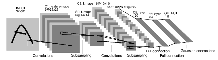
2. Defining a Convolutional Neural Network
import torch.nn as nn
import torch.nn.functional as F

class Net(nn.Module):    def __init__(self):        super(Net, self).__init__()        self.conv1 = nn.Conv2d(3, 6, 5)        self.pool = nn.MaxPool2d(2, 2)        self.conv2 = nn.Conv2d(6, 16, 5)        self.fc1 = nn.Linear(16 * 5 * 5, 120)        self.fc2 = nn.Linear(120, 84)        self.fc3 = nn.Linear(84, 10)
    def forward(self, x):        x = self.pool(F.relu(self.conv1(x)))        x = self.pool(F.relu(self.conv2(x)))        x = x.view(-1, 16 * 5 * 5)        x = F.relu(self.fc1(x))        x = F.relu(self.fc2(x))        x = self.fc3(x)        return x

net = Net()
3. Defining the Loss Function and Optimizer
import torch.optim as optim
criterion = nn.CrossEntropyLoss()
optimizer = optim.SGD(net.parameters(), lr=0.001, momentum=0.9)
4. Training the Network
for epoch in range(2):  # loop over the dataset multiple times
    running_loss = 0.0    for i, data in enumerate(trainloader, 0):        # get the inputs; data is a list of [inputs, labels]        inputs, labels = data
        # zero the parameter gradients        optimizer.zero_grad()
        # forward + backward + optimize        outputs = net(inputs)        loss = criterion(outputs, labels)        loss.backward()        optimizer.step()
        # print statistics        running_loss += loss.item()        if i % 2000 == 1999:    # print every 2000 mini-batches            print('[%d, %5d] loss: %.3f' %                  (epoch + 1, i + 1, running_loss / 2000))            running_loss = 0.0
print('Finished Training')
PATH = './cifar_net.pth'
torch.save(net.state_dict(), PATH)
5. Testing the Network on the Test Set
dataiter = iter(testloader)
images, labels = dataiter.next()
# print images
imshow(torchvision.utils.make_grid(images))
print('GroundTruth: ', ' '.join('%5s' % classes[labels[j]] for j in range(4)))
net = Net()
net.load_state_dict(torch.load(PATH))
outputs = net(images)
_, predicted = torch.max(outputs, 1)
print('Predicted: ', ' '.join('%5s' % classes[predicted[j]]                              for j in range(4)))
correct = 0
total = 0
with torch.no_grad():    for data in testloader:        images, labels = data        outputs = net(images)        _, predicted = torch.max(outputs.data, 1)        total += labels.size(0)        correct += (predicted == labels).sum().item()
print('Accuracy of the network on the 10000 test images: %d %%' % (    100 * correct / total))
class_correct = list(0. for i in range(10))
class_total = list(0. for i in range(10))
with torch.no_grad():    for data in testloader:        images, labels = data        outputs = net(images)        _, predicted = torch.max(outputs, 1)        c = (predicted == labels).squeeze()        for i in range(4):            label = labels[i]            class_correct[label] += c[i].item()            class_total[label] += 1
for i in range(10):    print('Accuracy of %5s : %2d %%' % (        classes[i], 100 * class_correct[i] / class_total[i]))
Training on GPU
device = torch.device("cuda:0" if torch.cuda.is_available() else "cpu")# Assume that we are on a CUDA machine, then this should print a CUDA device:#假设我们有一台CUDA的机器,这个操作将显示CUDA设备。print(device)
net.to(device)
Please remember that you must also convert your inputs and targets to the GPU at every step:
inputs, labels = inputs.to(device), labels.to(device)
Practice:
Goals Achieved:
-
Gained deeper understanding of PyTorch’s tensor library and neural networks -
Trained a small network to classify images
Training on Multiple GPUs
If you want to use all GPUs to speed things up even more, check out the further reading: [Data Parallelism]:
(https://pytorch.org/tutorials/beginner/blitz/data_parallel_tutorial.html)
What to do next?
-
Train a neural network to play video games -
Train the best ResNet on ImageNet -
Use generative adversarial networks to train a face generator -
Train a character-level language model using LSTM networks -
More examples -
More tutorials -
Discuss PyTorch on forums -
Chat with other users on Slack
https://github.com/fengdu78/machine_learning_beginner/tree/master/PyTorch_beginner
Editor: Yu Tengkai
Proofreader: Lin Yilin