Click the above“Beginner Learning Vision” to select “Star” or “Pin”
Heavyweight content delivered first-hand
Introduction
In recent years, there has been increasing interest in extending deep learning methods to graphs. Driven by multiple factors, researchers have drawn on ideas from convolutional networks, recurrent networks, and deep autoencoders to define and design neural network structures for processing graph data, giving rise to a new research hotspot—“Graph Neural Networks (GNN).”

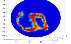
Figure 1: A graph from (Bruna et al., ICLR, 2014) depicting MNIST images in the 3D domain. While convolutional networks struggle to classify spherical data, graph networks can handle it quite naturally. It can be seen as a processing tool, but many similar tasks will arise in practical applications.
Author:Boris Knyazev
Translation:Li Feng
Recently, Graph Neural Networks (GNN) have become increasingly popular in various fields, including social networks, knowledge graphs, recommendation systems, and even life sciences. GNNs excel in modeling node relationships, leading to significant breakthroughs in related research areas. This article will discuss the questions of “Why are graphs useful?”, “Why is it challenging to define convolution on graphs?”, and “What transforms neural networks into graph neural networks?”.
First, let’s briefly review what a graph is. A graph G is a set of nodes (vertices) connected by directed or undirected edges. Nodes and edges are typically set by experts based on knowledge or intuition about the problem. Thus, they can represent atoms in molecules, users in social networks, cities in transportation systems, athletes in team sports, neurons in the brain, interacting objects in dynamic physical systems, pixels in images, image bounding boxes, or image segmentation masks.
In other words, in many cases, it’s really up to you to decide the nodes and edges of the graph.
This is a flexible data structure that encompasses many other data structures. For instance, without edges, it becomes a set; if there are only “vertical” edges, where any two nodes are connected, we have a data tree. Of course, as we will discuss next, this flexibility has both advantages and disadvantages.
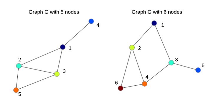
Figure 2: Two undirected graphs with 5 and 6 nodes, where the order of nodes is arbitrary.
1. Why Are Graphs Useful
In the context of computer vision (CV) and machine learning (ML), studying graphs and learning models can provide us with at least four benefits:
1. We have the opportunity to solve previously unsolvable problems, such as: cancer drug discovery (Veselkov et al., Nature, 2019); better understanding of human brain structure (Diez & Sepulcre, Nature, 2019); discovery of energy and environmentally friendly materials (Xie et al., Nature Communications, 2019).
2. In most CV/ML applications, you may have seen them as another data structure, but data can actually be viewed as graphs. Representing data as graphs can offer great flexibility and provide a completely different perspective when addressing problems. For instance, you can learn directly from “superpixels” instead of learning from image pixels, as evidenced in Liang et al.’s 2016 paper published in ECCV and our upcoming BMVC paper. Graphs also allow you to impose relational inductive biases on the data, enabling you to have some prior knowledge while solving problems. For example, if you want to reason about human posture, your relational bias could be a graph of human skeletal joints (Yen et al., AAAI, 2018); or if you want to reason about videos, your relational bias could be a graph of moving bounding boxes (Wang & Gupta, ECCV, 2018). Another example is representing facial landmarks as graphs (Antonakos et al., CVPR, 2015) for recognizing facial features and identities.
3. Neural networks themselves can be seen as a graph, where nodes are neurons, edges are weights, or nodes are layers, and edges represent the forward/backward flow (in this case, we are discussing computational graphs used in TensorFlow, PyTorch, and other DL frameworks). Applications can include optimization of computational graphs, neural architecture search, and training behavior analysis.
4. Finally, you can solve many problems more efficiently when the data can be naturally represented as a graph. This includes but is not limited to classification of molecular and social networks (Knyazev et al., NeurIPS-W, 2018), classification and correspondence of 3D meshes (Fey et al., CVPR 2018), modeling behavior of dynamic interacting objects (Kipf et al., ICML, 2018), scene graph modeling (see the upcoming ICCV workshop), question answering (Narasimhan, NeurIPS, 2018), program synthesis (Allamanis et al., ICLR, 2018), various reinforcement learning tasks (Bapst et al., ICML, 2019), and many other problems.
I previously researched facial recognition and facial emotion analysis, so I appreciate the following graph.
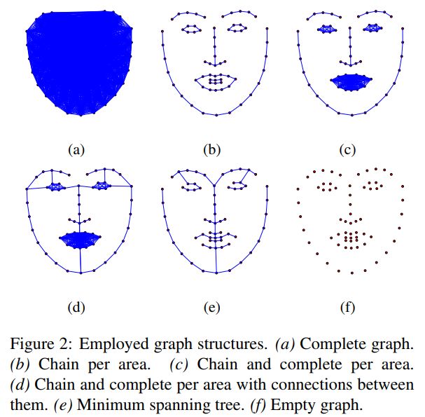
Figure 3: A graph from (Antonakos et al., CVPR, 2015) extracting facial landmarks. This is an interesting approach, but in many cases, it does not comprehensively represent a person’s facial features, so more information can be captured from facial textures through convolutional networks. In contrast, reasoning based on a 3D mesh of a face appears more reasonable compared to 2D landmarks (Ranjan et al., ECCV, 2018).
2. Why Is It Difficult to Define Convolution on Graphs
To answer this question, we first need to clarify the general motivation for using convolution and then describe “convolution on images” using graph terminology, which will make the transition to “graph convolution” smoother.
1. Why Is Convolution Useful
We should understand why we pay attention to convolution and why we want to use it to process graphs. Compared to fully connected neural networks (NNS or MLP), convolutional networks (CNN or Convnet) have certain advantages.
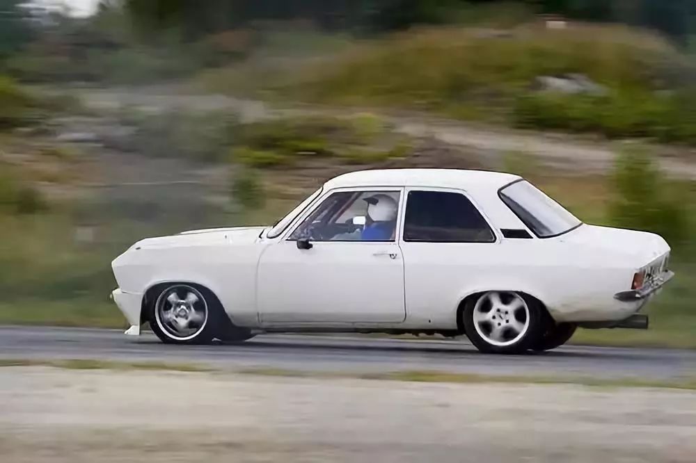
Figure 4
First, Convnet utilizes a natural prior in images, which has been more formally described in Bronstein et al.’s 2016 paper, for example:
(1) Translation invariance, if we translate the car in the above image left/right/up/down, we can still recognize it as a car. This is achieved by sharing filters across all positions, that is, applying convolution.
(2) Locality, nearby pixels are closely related and usually represent some semantic concepts like wheels or windows. This is achieved by using relatively large filters that can capture image features in the local spatial neighborhood.
(3) Compositionality (or hierarchy), larger areas in images usually contain semantic parents of smaller areas. For example, a car is the parent of doors, windows, wheels, and the driver, while the driver is the parent of the head, arms, etc. This is achieved through stacking convolutional layers and applying pooling for implicit representation.
Secondly, the number of trainable parameters (i.e., filters) in convolutional layers does not depend on the input dimensions, so technically we can train the same model on 28×28 and 512×512 images. In other words, the model is parameterized.
Ideally, our goal is to develop a model as flexible as a graph neural network that can digest and learn any data, but at the same time, we want to control (regularize) the elements of this flexibility by turning certain priors on or off.
All these good properties make ConvNet less prone to overfitting (high accuracy on the training set and low accuracy on validation/testing sets), more accurate across different vision tasks, and easier to scale to large images and datasets. Therefore, when we want to solve important tasks where the input data is graph-structured, we transfer all these attributes to Graph Neural Networks (GNN) to regularize their flexibility and make them scalable. Ideally, our goal is to develop a model as flexible as a GNN that can digest and learn any data, but we also want to control (regularize) the elements of this flexibility by turning certain priors on or off. This can be researched in many innovative directions. However, achieving control and reaching a balanced state is still quite challenging.
2. Performing Convolution on Graphs
Let’s first consider an undirected graph G with N nodes, where edges E represent undirected connections between nodes. Nodes and edges are typically set by yourself. Regarding images, we consider nodes to be pixels or superpixels (a group of oddly shaped pixels), and edges to represent their spatial distances. For example, the MNIST image in the lower left corner is typically represented as a 28×28 dimensional matrix. We can also represent it with a set of N=28*28=784 pixels. Therefore, our graph G should have N=784 nodes, and for closely located pixels, the edges will have a larger value (thicker edges in the figure below), while for distant pixels, the corresponding values will be smaller (thinner edges).

Figure 5: On the left is an image from the MNIST dataset, and on the right is a demonstration of the graph. The darker and larger nodes on the right correspond to higher pixel intensities. The right graph is inspired by Figure 6 (Fey et al., CVPR, 2018).
When we train a neural network or Convnet on an image, we subconsciously define the image on a regular 2D grid, as shown in the figure below. This grid is the same and regular for all training and testing images, meaning all pixels in the grid are connected in exactly the same way across all images (i.e., having the same number of connections, edge lengths, etc.), so this regular grid graph cannot help us distinguish one image from another. Below I visualize some 2D and 3D regular grids, where the order of nodes is color-coded. By the way, I implemented this in Python code using NetworkX, for example G=networkx.Grid_Graph([4,4]).
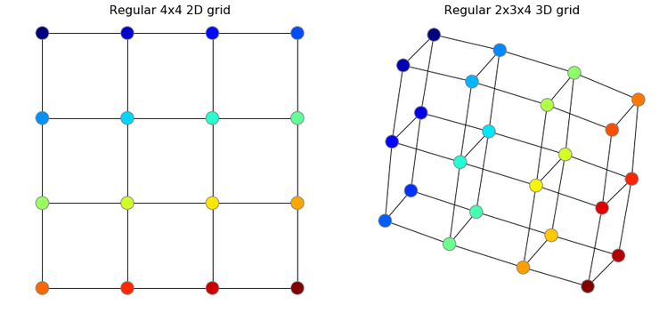
Figure 6: Examples of regular 2D and 3D grids. Representation of images on a 2D grid, and videos on a 3D grid.
Considering this is a 4×4 regular grid, we can simply look at how 2D convolution works to understand why it’s difficult to translate operators into graphs. Filters on regular grids have the same node levels, but modern convolutional networks often have small filters, such as the 3×3 in the example below. This filter has 9 values: W₁, W₂, …, W₉, which are updated during training using the backpropagation tool to minimize loss and solve downstream tasks. In the example below, we are inspired to initialize the filter as an edge detector (see here for other possible filters):

Figure 7: An example of a 3×3 filter on a regular 2D grid, where the left side has arbitrary weights w, and the right side is an edge detector.
When we perform convolution, we slide this filter in two directions: right and down, starting from the bottom corner, and it’s important to slide through all possible positions. At each position, we calculate the dot product between the values on the grid (denoted as X) and the filter values W: X₁W₁+X₂W₂+…+X₉W₉, and store the result in the output image. In our visualization process, we change the color of the nodes during the sliding process to match the colors of the nodes in the grid. In regular grids, we always match the nodes of the filter with the nodes of the grid. But this does not apply to graphs, and I will explain below.
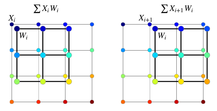
Figure 8: Two steps of 2D convolution on a regular grid. If we do not apply padding, there will be a total of 4 steps, resulting in a 2×2 image. To make the resulting image larger, we need to apply padding. Here, please refer to the comprehensive guide on convolution in deep learning.
The dot product used above is one of the so-called “aggregation operators.” Broadly speaking, the goal of aggregation operators is to summarize data into simpler forms. In the above example, the dot product summarizes a 3×3 matrix into a single value. Another example is data summarization in Convnet. Remember, positions like maximum or sum total values are invariant, meaning even if all pixels in that area are randomly moved, they will still summarize to the same value in the spatial area. To illustrate this, the dot product is not permutation invariant because in general: X₁W₁+X₂W₂≠X₂W₁+X₁W₂.
Now, let’s use the MNIST image to define the regular grid, filter, and convolution. Considering our graph terminology, this regular 28×28 grid will be our graph G, so each cell in this grid is a node, and the node feature is an actual image X, meaning each node has only one feature, with pixel intensity ranging from 0 (black) to 1 (white).

Figure 9: Regular 28×28 grid (left) and the image on that grid (right).
Next, we will define the filter and make it a famous Gabor filter with (almost) arbitrary parameters. Once we have the image and the filter, we can perform convolution by sliding the filter over the image (in our case, the number 7) and placing the dot product result into the output matrix at each step.
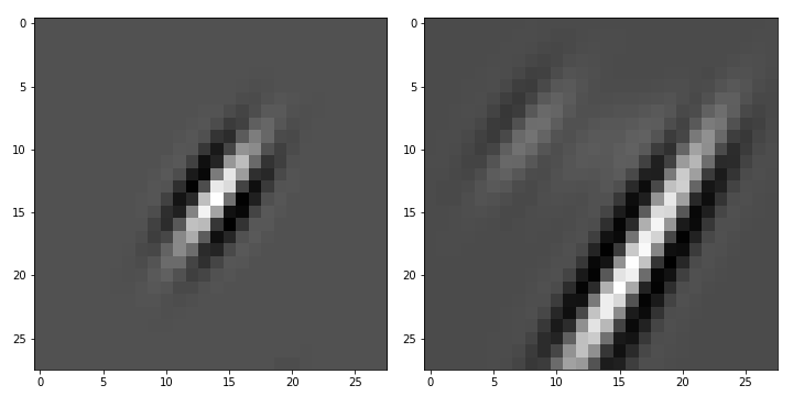
Figure 10: A 28×28 filter (left) and the result of the 2D convolution of that filter with the digit 7 image (right).
As I mentioned earlier, when you try to apply convolution to graphs, you encounter many issues.
Nodes are a set, and any permutation of that set does not change it. Therefore, the aggregation operators applied should be permutation invariant.
As I mentioned earlier, the dot product used to compute each step of convolution is sensitive to order. This sensitivity enables us to learn edge detectors similar to Gabor filters, which are essential for capturing image features. The problem is that there is no clearly defined node order in graphs unless you learn to sort them or come up with some other heuristic methods that can form a normative order between graphs. In short, nodes are a set, and any permutation of that set does not change it. Therefore, the aggregation operators applied should be permutation invariant. The most popular choices are the mean (GCN, Kipf & Wling, ICLR, 2017) and summing all adjacent values (GIN, Xu et al., ICLR, 2019), which is the summation or mean pooling, then inferred by a trainable vector W, for other aggregators see Hamilton et al., NIPS, 2017.

Figure 11: Illustrating “graph convolution” of node features X, with filter W centered at node 1 (deep blue).
For example, in the left graph, the output of the summing aggregator at node 1 would be X₁=(X₁+X₂+X₃+X₄)W₁, for node 2: X₂=(X₁+X₂+X₃+X₅)W₁, etc., meaning we need to apply this aggregator to all nodes. Thus, we will get a graph with the same structure, where nodes now contain the features of all neighboring values. We can handle the right graph in the same way.
Colloquially, this averaging or summation is referred to as “convolution” because we also “slide” from one node to another and apply the aggregation operator at each step. However, the important point is that this is a very special form of convolution, where the filter has no directional sense. Below, I will show what these filters look like and provide suggestions on how to improve them.
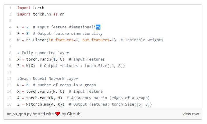
3. What Makes Neural Networks into Graph Neural Networks
You should know how a typical neural network works, where we take C-dimensional features X as input to the network. Using MNIST as an example, X would be our C=784 dimensional pixel features (i.e., “flattened” images). These features multiply by weights W of dimensions C×F, updated during training, to make the output closer to our expected result. This result can be directly used to solve tasks (for example, in regression cases) or can be further fed back into some non-linear (activation), such as relu, or other differentiable (or more accurately, sub-differentiable) functions, forming a multi-layer network. Generally, the output of layer l is:

Figure 12: Fully connected layer with learnable weights W. “Fully connected” means every output value in X⁽ˡ⁺1 1⁾ depends on or is “connected to” all inputs X⁽ˡ⁾. Typically, although not always, we also add a bias term in the output.
The signals in MNIST are very strong, and just using the formula above and cross-entropy loss, the accuracy can exceed 91% without any non-linearities or other tricks (I achieved this using a slightly modified PyTorch code). This model is referred to as polynomial (or multiclass, since we have 10 classes of digits) logistic regression.
Now, how do we convert our neural network into a graph neural network? As you already know, the core idea behind GNN is to aggregate “neighboring values.” Here, the key point is to understand that in many cases, it is actually you who specify the “neighboring values.”
Let’s first consider a simple case when you have some graphs. For example, this could be a fragment (subgraph) of a social network of 5 people, where edges between nodes indicate whether two people are friends (or at least one of them thinks so). The adjacency matrix on the right graph (usually denoted as A) is a way to represent these edges in matrix form, making it easier to construct our deep learning framework. Yellow in the matrix represents edges, while blue represents missing edges.
Figure 13: An example of a graph and its adjacency matrix. The order of nodes defined in both cases is random, while the graph remains the same.
Now, let’s create an adjacency matrix A for our MNIST example based on the coordinates of pixels (the complete code is provided at the end of the article):
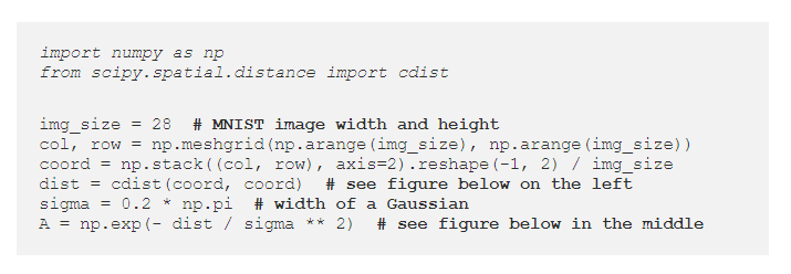
This is a typical method of defining adjacency matrices in visual tasks, but it is not the only method (Defferrard et al., 2016; Bronstein et al., 2016). This adjacency matrix is our prior, or our inductive bias, which we impose on the model based on experience, assuming that nearby pixels should be connected, while distant pixels should not have edges, and if they do, the edges should be very thin (small value edges). This is because we observe that neighboring pixels in natural images usually correspond to the same or multiple frequently interacting objects (the locality principle we mentioned earlier), so it makes sense to connect these pixels.
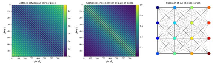
Figure 14: Distances between all node pairs in the adjacency matrix (left) and the adjacency matrix (middle) (right) with a subgraph of 16 neighboring pixels corresponding to the middle adjacency matrix. Since it is a complete subgraph, it is also referred to as a “cluster.”
So now there are not only features X but also some peculiar matrix A with values in the range [0,1]. It is important to note that once we know the input is a graph, we assume that the order of all other graph nodes in the dataset is consistent. In terms of images, this means assuming that pixels are randomly shuffled. In practice, finding a normative order for nodes is fundamentally unsolvable. Although for MNIST, we can operate under this assumption (since the data originally comes from a regular grid), it does not apply to actual graph datasets.
Remember, our feature matrix X has N rows and C columns. Thus, in terms of graphs, each row corresponds to a node, and C is the dimension of node features. But now the question is, we do not know the order of nodes, so we do not know where to place the features of specific nodes in which row.
If we simply ignore this issue and provide X directly to the MLP as before, it would be equivalent to forming an image by randomly shuffling pixels (and don’t forget to adjust A in the same way), surprisingly, neural networks can fit such random data in principle (Zhang et al., ICLR, 2017), but the testing performance will approach random predictions. One solution is to simply use the previously created adjacency matrix A, as follows:
 Figure 16. Graph neural layer with adjacency matrix A, input or output features X, and learnable weights W.
We just need to ensure that the first row in A corresponds to the features of the first row in X for the nodes. Here, I am using 𝓐 instead of the regular A because you want to normalize A, if 𝓐=A, the matrix multiplication 𝓐X⁽ˡ⁾ will be equivalent to summing features of neighboring values, which is useful in many tasks (Xu et al., ICLR, 2019). The most common case is that you normalize it so that 𝓐X⁽ˡ⁾ has the properties of averaging neighboring values, i.e., 𝓐=A/ΣᵢAᵢ. Better methods for normalizing matrix A can be found in (Kipf & Wling, ICLR, 2017).
Below is a comparison of NN and GNN in terms of PyTorch code:
Here is the complete PyTorch code to train the two models above: Python mnist_fc.py – model fc trains the NN model; python mnist_fc.py – model graph trains the GNN model. As an exercise, you can try to randomly shuffle the pixels in the model graph in the code (don’t forget to adjust A in the same way) and see if it doesn’t affect the results. Would it be feasible for the FC model?
After running the code, you may notice that the classification accuracy is actually the same. So what’s the problem? Shouldn’t graph networks perform better? In fact, in most cases, they work just fine, but in this case, there is a special situation because the operator we added 𝓐X⁽ˡ⁾ is essentially a Gaussian filter:
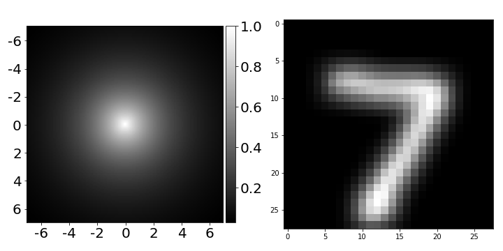
Figure 17: 2D visualization of filters in graph neural networks and their effects on images.
Our graph neural network has been shown to be equivalent to a convolutional neural network with a single Gaussian filter, which we never update during training, followed by fully connected layers. This filter essentially displays a blurred or clear image, which is not particularly useful (see the right side of the above image). However, this is the simplest variant of graph neural networks, and still, it performs well on graph-structured data. To make GNNs work better on regular graphs (like images), we need to apply some tricks. For example, we can learn to predict edges between any pair of pixels using a differentiable function instead of using predefined Gaussian filters:
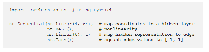
To make GNNs work better on regular graphs (like images), we need to apply some tricks. For example, we can learn to predict edges between any pair of pixels using a differentiable function instead of using predefined Gaussian filters.
This idea is similar to dynamic filter networks (Brabander et al., NIPS, 2016), edge-conditioned graph networks (ECC, Simonovsky & Komodakis, CVPR, 2017), and (Knyazev et al., NeurIPS-W, 2018). If you want to try it with our code, you can simply add the -pred_Edge flag, so the complete command would be python mnist_fc.py –model graph –pred_edge. Below, I show the animation of predefined Gaussian filters and learned filters. You may notice that the learned filters (in the middle) look strange. This is because the task is quite complex, and we are optimizing two models simultaneously: the model for predicting edges and the model for predicting digit classes. To better learn the filters (as shown on the right), we need to apply some additional techniques from the BMVC paper, which is beyond the scope of this tutorial.
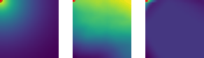
Figure 18: 2D neural network filter centered on a red dot. Average (left 92.2 4%), coordinate learning (middle 91.05%), coordinate learning (right 92.39%).
The code to generate these GIFs is very simple:

I also shared an IPython notebook that shows the 2D convolution of images using Gabor filters (using adjacency matrices) instead of using convolution matrices, which are typically used in signal processing.
In the next part of this tutorial, I will detail more advanced graph layers that can better filter graphs.
4. Conclusion
Graph neural networks are a very flexible and interesting family of neural networks that can be applied to very complex data. Of course, this flexibility comes at a cost. In the case of GNNs, it is challenging to regularize the model by defining such operators as convolutions. However, research in this area is progressing rapidly, and it is believed that a comprehensive solution will soon be achieved, and GNNs will find increasingly widespread applications in machine learning and computer vision.
via : https://medium.com/@BorisAKnyazev/tutorial-on-graph-neural-networks-for-computer-vision-and-beyond-part-1-3d9fada3b80d
Group Chat
Welcome to join the public account reader group to exchange ideas with peers. Currently, there are WeChat groups on SLAM, 3D vision, sensors, autonomous driving, computational photography, detection, segmentation, recognition, medical imaging, GAN, algorithm competitions, etc. (will gradually be subdivided in the future), please scan the WeChat number below to join the group, and note: “nickname + school/company + research direction”, for example: “Zhang San + Shanghai Jiao Tong University + Vision SLAM”. Please follow the format, otherwise it will not be approved. After successfully adding, you will be invited to join the relevant WeChat group based on your research direction. Please do not send advertisements in the group, or you will be removed from the group, thank you for your understanding~