Click the above “Beginner’s Guide to Vision” to select “Star” or “Top”
Heavyweight content delivered first-hand

This article is sourced from | Visual Algorithms
Don’t let your neural network end up like this
Let’s face it, your model might still be stuck in the Stone Age. I bet you’re still using 32-bit precision or GASP even training on just one GPU.
I understand that there are various neural network acceleration guides online, but there isn’t a checklist (now there is). Use this checklist to ensure you can squeeze out all the performance from your model step by step.
This guide covers changes from the simplest structures to the most complex modifications that can maximize the benefits for your network. I will show you example PyTorch code and relevant flags that can be used with the PyTorch-Lightning Trainer, so you don’t have to write this code yourself!
Who is this guide for? Anyone conducting deep learning model research using PyTorch, such as researchers, PhD students, scholars, etc. The models we are discussing here may require days, weeks, or even months of training.
-
-
Number of workers in DataLoader
-
-
-
Retained computation graph
-
-
16-bit mixed precision training
-
Moving to multiple GPUs (model replication)
-
Moving to multiple GPU nodes (8+ GPUs)
-
Thinking about model acceleration tips
You can find every optimization I discuss here in the PyTorch library Pytorch-lightning. Lightning is a wrapper on top of PyTorch that can automate training while giving researchers full control over key model components. Lightning uses the latest best practices and minimizes the chances of errors.
We define LightningModel for MNIST and use Trainer to train the model.
from pytorch_lightning import Trainer
model = LightningModule(…)
trainer = Trainer()
trainer.fit(model)


1.DataLoaders
This might be the easiest place to gain speed. The era of saving h5py or numpy files to speed up data loading is long gone; using the PyTorch DataLoader to load image data is straightforward (for NLP data, check out TorchText).
In Lightning, you don’t need to specify the training loop; just define the dataLoaders and Trainer will call them when needed.
dataset = MNIST(root=self.hparams.data_root, train=train, download=True)
loader = DataLoader(dataset, batch_size=32, shuffle=True)
for batch in loader:
  x, y = batch
  model.training_step(x, y)
  ...


2.Number of workers in DataLoader
Another magical acceleration point is allowing batch parallel loading. Thus, you can load nb_workers batches at once instead of one batch at a time.
# slow
loader = DataLoader(dataset, batch_size=32, shuffle=True)
# fast (use 10 workers)
loader = DataLoader(dataset, batch_size=32, shuffle=True, num_workers=10)


3.Batch size
Before starting the next optimization step, increase the batch size to the maximum allowed by CPU-RAM or GPU-RAM.
The next section will focus on how to help reduce memory usage so you can continue to increase the batch size.
Remember, you may need to update your learning rate again. A good rule of thumb is that if the batch size doubles, then the learning rate doubles.
If your batch size is still too small (like 8) when you have already reached the limit of computational resources, then we need to simulate a larger batch size for gradient descent to provide a good estimate.
Suppose we want to achieve a batch size of 128. We need to perform 16 forward and backward passes with a batch size of 8 and then execute one optimization step.
# clear last step
optimizer.zero_grad()

# 16 accumulated gradient steps
scaled_loss = 0
for accumulated_step_i in range(16):
     out = model.forward()
     loss = some_loss(out,y)
     loss.backward()
      scaled_loss += loss.item()

# update weights after 8 steps. effective batch = 8*16
optimizer.step()

# loss is now scaled up by the number of accumulated batches
actual_loss = scaled_loss / 16
In Lightning, it’s all done for you; just set <span>accumulate_grad_batches=16</span>:
trainer = Trainer(accumulate_grad_batches=16)
trainer.fit(model)


5.Retained Computation Graph
One of the simplest ways to blow up your memory is to log your loss.
losses = []
...
losses.append(loss)

print(f'current loss: {torch.mean(losses)}')
The problem above is that loss still contains a copy of the entire graph. In this case, call .item() to release it.
# bad
losses.append(loss)
# good
losses.append(loss.item())
Lightning will be very careful to ensure that a copy of the computation graph is not retained.
Once you’ve completed the previous steps, it’s time to move to GPU training. Training on a GPU will parallelize the mathematical computations across multiple GPU cores. The speedup you get depends on the type of GPU you are using. I recommend using a 2080Ti for personal use and a V100 for companies.
At first glance, this may seem overwhelming, but you really only need to do two things: 1) Move your model to the GPU, 2) Whenever you run data through it, put the data on the GPU.
# put model on GPU
model.cuda(0)

# put data on gpu (cuda on a variable returns a cuda copy)
x = x.cuda(0)

# runs on GPU now
model(x)
If you are using Lightning, you don’t have to do anything; just set <span>Trainer(gpus=1)</span>.
# ask lightning to use gpu 0 for training
trainer = Trainer(gpus=[0])
trainer.fit(model)
When training on a GPU, the main thing to keep in mind is to limit the number of transfers between the CPU and GPU.
# expensive
x = x.cuda(0)# very expensive
x = x.cpu()
x = x.cuda(0)
If memory runs out, do not move data back to the CPU to save memory. Before resorting to the GPU, try optimizing your code or memory distribution between GPUs in other ways.
Another thing to be aware of is calling operations that force GPU synchronization. Clearing memory cache is one example.
# really bad idea. Stops all the GPUs until they all catch up
torch.cuda.empty_cache()
However, if you are using Lightning, the only place where issues may arise is when defining the Lightning Module. Lightning is particularly careful not to make these kinds of mistakes.
16-bit precision is an amazing technique that halves memory usage. Most models are trained using 32-bit precision numbers. However, recent research has found that 16-bit models can also work quite well. Mixed precision means using 16-bit for some things while keeping weights and other things at 32-bit.
To use 16-bit precision in PyTorch, install NVIDIA’s apex library and make these changes to your model.
# enable 16-bit on the model and the optimizer
model, optimizers = amp.initialize(model, optimizers, opt_level='O2')

# when doing .backward, let amp do it so it can scale the loss
with amp.scale_loss(loss, optimizer) as scaled_loss:
    scaled_loss.backward()
The amp package will handle most things. If gradients explode or trend toward zero, it will even scale the loss.
In Lightning, enabling 16-bit does not require any modifications to the model or executing the operations I mentioned above. Just set <span>Trainer(precision=16)</span>.
trainer = Trainer(amp_level='O2', use_amp=False)
trainer.fit(model)


8.Moving to Multiple GPUs
Now things get really interesting. There are three (maybe more?) ways to do multi-GPU training.
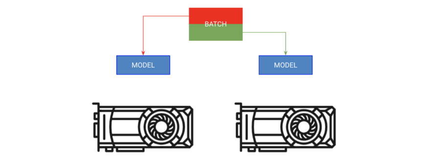
A) Copy the model to each GPU, B) Give each GPU a portion of the batch
The first method is called “batch splitting training.” This strategy replicates the model on each GPU, with each GPU receiving a portion of the batch.
# copy model on each GPU and give a fourth of the batch to each
model = DataParallel(model, devices=[0, 1, 2 ,3])

# out has 4 outputs (one for each gpu)
out = model(x.cuda(0))
In Lightning, you just need to increase the number of GPUs and tell the trainer; you don’t have to do anything else.
# ask lightning to use 4 GPUs for training
trainer = Trainer(gpus=[0, 1, 2, 3])
trainer.fit(model)
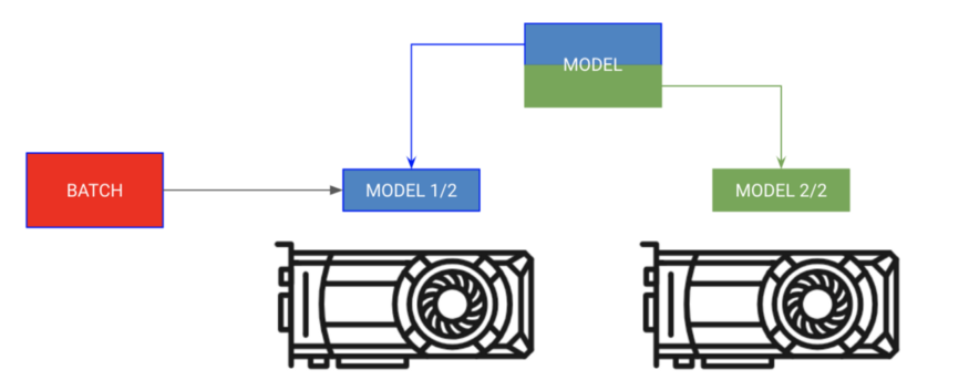
Model Distribution Training
Place different parts of the model on different GPUs, with the batch moving in sequence
Sometimes your model may be too large to fit entirely in memory. For example, a sequence-to-sequence model with an encoder and decoder may occupy 20GB of RAM when generating outputs. In this case, we want to place the encoder and decoder on separate GPUs.
# each model is sooo big we can't fit both in memory
encoder_rnn.cuda(0)
decoder_rnn.cuda(1)

# run input through encoder on GPU 0
encoder_out = encoder_rnn(x.cuda(0))

# run output through decoder on the next GPU
out = decoder_rnn(encoder_out.cuda(1))

# normally we want to bring all outputs back to GPU 0
out = out.cuda(0)
For this type of training, in Lightning, you don’t need to specify any GPUs; you should place the modules in the LightningModule on the correct GPUs.
class MyModule(LightningModule):
    def __init__():
        self.encoder = RNN(...)
        self.decoder = RNN(...)
    def forward(x):
        # models won't be moved after the first forward because
        # they are already on the correct GPUs
        self.encoder.cuda(0)
        self.decoder.cuda(1)
        out = self.encoder(x)
        out = self.decoder(out.cuda(1))

# don't pass GPUs to trainer
model = MyModule()
trainer = Trainer()
trainer.fit(model)
In the above case, the encoder and decoder can still benefit from parallelization.
# change these lines
self.encoder = RNN(...)
self.decoder = RNN(...)

# to these
# now each RNN is based on a different gpu set
self.encoder = DataParallel(self.encoder, devices=[0, 1, 2, 3])
self.decoder = DataParallel(self.encoder, devices=[4, 5, 6, 7])

# in forward...
out = self.encoder(x.cuda(0))

# notice inputs on first gpu in device
sout = self.decoder(out.cuda(4))  # <--- the 4 here
Considerations when using multiple GPUs:
-
If the model is already on the GPU, model.cuda() does nothing.
-
Always place the input on the first device in the device list.
-
Transferring data between devices is expensive; treat it as a last resort.
-
Optimizers and gradients will be saved on GPU 0, so the memory used on GPU 0 may be significantly larger than on other GPUs.
9.Multi-Node GPU Training
Each GPU on each machine has a copy of the model. Each machine receives a portion of the data and trains only on that portion. Each machine can synchronize gradients.
If you’ve made it this far, then you can now train Imagenet in just a few minutes! It’s not as difficult as you might imagine, but it may require more knowledge about compute clusters. These instructions assume you are using SLURM on a cluster.
PyTorch allows multi-node training by replicating the model on each GPU in each node and synchronizing gradients. So, each model is independently initialized on each GPU and essentially trains independently on a partition of the data, except they all receive gradient updates from all models.
-
Initialize a copy of the model on each GPU (make sure to set the seed so that each model initializes to the same weights, or it will fail).
-
Split the dataset into subsets (using DistributedSampler). Each GPU trains only on its own small subset.
-
On .backward(), all replicas receive a copy of the gradients from all models. This is the only communication between models.
PyTorch has a great abstraction called DistributedDataParallel that can help you achieve this. To use DDP, you need to do 4 things:
def tng_dataloader():
     d = MNIST()

     # 4: Add distributed sampler
     # sampler sends a portion of tng data to each machine
     dist_sampler = DistributedSampler(dataset)
     dataloader = DataLoader(d, shuffle=False, sampler=dist_sampler)

def main_process_entrypoint(gpu_nb):
     # 2: set up connections  between all gpus across all machines
     # all gpus connect to a single GPU "root"
     # the default uses env://
     world = nb_gpus * nb_nodes
     dist.init_process_group("nccl", rank=gpu_nb, world_size=world)

     # 3: wrap model in DPP
     torch.cuda.set_device(gpu_nb)
     model.cuda(gpu_nb)
     model = DistributedDataParallel(model, device_ids=[gpu_nb])

     # train your model now...

if  __name__ == '__main__':
     # 1: spawn number of processes
     # your cluster will call main for each machine
     mp.spawn(main_process_entrypoint, nprocs=8)
However, in Lightning, you just need to set the number of nodes, and it will handle the rest for you.
# train on 1024 gpus across 128 nodes
trainer = Trainer(nb_gpu_nodes=128, gpus=[0, 1, 2, 3, 4, 5, 6, 7])
Lightning also comes with a SlurmCluster manager to conveniently help you submit the correct details for SLURM jobs.
10.Benefit! Faster Training on a Single Node with Multiple GPUs
It turns out that DistributedDataParallel is much faster than DataParallel because it only performs the communication for gradient synchronization. So, a good hack is to use DistributedDataParallel instead of DataParallel, even when training on a single machine.
In Lightning, this is easily achieved by setting the distributed_backend to ddp and setting the number of GPUs.
# train on 4 gpus on the same machine MUCH faster than DataParallel
trainer = Trainer(distributed_backend='ddp', gpus=[0, 1, 2, 3])
Although this guide will provide you with a series of tips to speed up your network, I still want to explain how to think about the problem by looking for bottlenecks.
I break the model into several parts:
First, I want to ensure there are no bottlenecks in data loading. To do this, I used the existing data loading solutions I described, but if none of these solutions meet your needs, consider offline processing and caching to high-performance data storage like h5py.
Next, look at what you are doing in the training step. Ensure that your forward pass is fast, avoid excessive computations, and minimize data transfers between the CPU and GPU. Finally, avoid doing things that will slow down the GPU (as discussed in this guide).
Next, I try to maximize my batch size, which is usually limited by the size of GPU memory. Now, I need to focus on how to distribute across multiple GPUs while using a large batch size and minimizing latency (for example, I might try using an effective batch size of 8000+ across multiple GPUs).
However, you need to be careful with large batch sizes. Refer to the relevant literature for your specific problem and see what people have overlooked!
Original article: https://towardsdatascience.com/9-tips-for-training-lightning-fast-neural-networks-in-pytorch-8e63a502f565
Good news, the knowledge platform of the Beginner’s Guide to Vision team is now open! To thank everyone for their support and love, the team has decided to grant free access to the knowledge platform worth 149 yuan. Everyone should seize the opportunity!

Download 1: OpenCV-Contrib Extension Module Chinese Tutorial
Reply in the backend of the “Beginner’s Guide to Vision” public account: Extension Module Chinese Tutorial, to download the first OpenCV extension module tutorial in Chinese on the internet, covering installation of extension modules, SFM algorithms, stereo vision, object tracking, biological vision, super-resolution processing, and more than twenty chapters of content.
Download 2: Python Vision Practical Project 52 Lectures
Reply in the “Beginner’s Guide to Vision” public account backend: Python Vision Practical Project, to download 31 visual practical projects including image segmentation, mask detection, lane line detection, vehicle counting, eyeliner addition, license plate recognition, character recognition, emotion detection, text content extraction, face recognition, etc., to assist in quickly learning computer vision.
Download 3: OpenCV Practical Project 20 Lectures
Reply in the “Beginner’s Guide to Vision” public account backend: OpenCV Practical Project 20 Lectures, to download 20 practical projects based on OpenCV to achieve advanced learning in OpenCV.
Group Chat
Welcome to join the public account reader group to exchange with peers. Currently, there are WeChat groups on SLAM, 3D vision, sensors, autonomous driving, computational photography, detection, segmentation, recognition, medical imaging, GAN, algorithm competitions, etc. (will gradually be subdivided in the future), please scan the WeChat number below to join the group, with the note: “nickname + school/company + research direction”, for example: “Zhang San + Shanghai Jiao Tong University + Vision SLAM”. Please follow the format for the note, otherwise, it will not be approved. After successfully adding, you will be invited to the relevant WeChat group based on your research direction. Please do not send advertisements in the group, otherwise, you will be removed from the group. Thank you for your understanding~