All algorithms in machine learning rely on minimizing or maximizing a function, which we call the “objective function.” The function that is minimized is called the “loss function,” which measures the model’s ability to predict the expected outcome. The most commonly used method for minimizing the loss function is the “gradient descent method.” You can think of the loss function as a hilly terrain, and gradient descent is like sliding down the hill to reach the lowest point.
No single loss function is suitable for all types of data; it depends on many factors, including the presence of outliers, the choice of machine learning algorithm, the time efficiency of gradient descent, and the confidence of predictions. The purpose of this article is to understand the different loss functions and how they help data scientists.
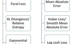
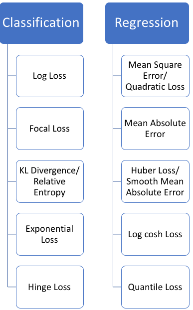
Loss functions can generally be divided into two categories: classification loss and regression loss. Regression functions predict quantities, while classification functions predict labels. The commonly used regression loss functions and classification loss functions are shown in the figure below:
In this article, I will mainly introduce regression loss functions.
Regression Loss
1. Mean Squared Error, Quadratic Loss, L2 Loss
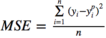
Mean Squared Error (MSE) is the most commonly used regression loss function. MSE is the sum of the squared distances between the target variable and the predicted values, and the formula is as follows:
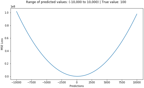
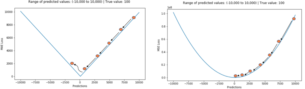
Below is a graph of the MSE function, where the true target value is 100, and the predicted values range from -10000 to 1000. The MSE loss value (y-axis) reaches its minimum when the prediction (x-axis) = 100, with the loss ranging from 0 to ∞.
2. Mean Absolute Error, L1 Loss
Mean Absolute Error (MAE) is another loss function used for regression models. MAE is the average of the absolute differences between the target values and the predicted values.
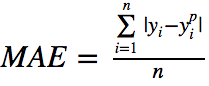
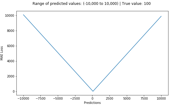
The MAE loss function curve is shown below:
Comparison of MSE and MAE (Comparison of L2 Loss and L1 Loss)
In short, using squared error is easier to solve, but using absolute error is more robust. Let’s see why.
When we train a machine learning model, our goal is to find the point that minimizes the loss function. Of course, both functions reach their minimum when the predicted value is exactly equal to the true value.
Below is a quick implementation of the two methods in Python. We can write our own functions or use the built-in metric functions from sklearn:
# true: Array of true target variable
# pred: Array of predictions
def mse(true, pred):
return np.sum((true - pred)**2)
def mae(true, pred):
return np.sum(np.abs(true - pred))
# also available in sklearn
from sklearn.metrics import mean_squared_error
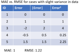
from sklearn.metrics import mean_absolute_errorLet’s compare the values of MAE and RMSE in two cases, where RMSE is the square root of MSE, making RMSE and MAE comparable on the same scale.
In the first case shown in the figure below, the predicted values are close to the true values, and the variance of the errors between the observations is small:
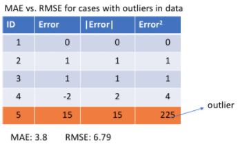
In the second case shown in the figure below, outliers appear between the observations, resulting in large errors.
What do we observe from this? How does it help us choose which loss function to use?
Since MSE squares the error (y – y_predicted = e), if e is greater than 1, the error (e) will increase significantly. If we have an outlier, the value of e will greatly increase, and the value of MSE will be far greater than e, which will give the MSE loss model more weight on the discrete values than the MAE loss model. If we adjust the model using RMSE as the loss, the loss model will minimize the outlier at the expense of other observations, which will reduce its overall performance.
If the training data is corrupted by outliers, MAE loss is useful, that is we have collected unrealistically large negative and positive values in the training data, rather than in the testing environment.
To put it intuitively, we can think like this: if we only need to give a prediction for all observations trying to minimize MSE, that prediction should be the average of all target values. But if we try to minimize MAE, that prediction would be the median of all observations. It is not hard to see that the median is more robust to outliers than the average, thus making MAE more robust to outliers than MSE.
A major issue with the MAE loss function is that its gradient is always the same, meaning that even when the loss value is small, the gradient can still be large. This is not beneficial for the model learning process. To address this issue, we can use a dynamic learning rate that decreases as we approach the minimum. MSE performs well in this case, even converging with a fixed learning rate. When the loss value is large, the gradient of MSE loss is high; when the loss approaches 0, the gradient of MSE loss decreases, making it more precise at the end of training (as shown in the figure below).
How to choose which loss function to use
If outliers represent something important for the business, we should use MSE; on the other hand, if we believe that outliers simply represent useless data, we should choose MAE as the loss function, with MAE and MSE also referred to as L1 and L2 losses, respectively.
Problems with both MAE and MSE
In some cases, neither of the two loss functions can provide satisfactory predictions. For example, if 90% of the target values in our data are 150, while the remaining 10% are between 0 and 30. Then, a model using MAE as the loss predicts all observations as 150, ignoring the 10% of outliers, as the model’s function approaches the median algorithm.
In the same situation, a model using MSE will give many predictions in the range of 0-30 because it will be skewed towards the outliers. In many business cases, both results are undesirable.
What to do in this case?
A simple solution is to transform the target variable; another method is to try a different loss function, which motivates the introduction of the third loss function: Huber loss.
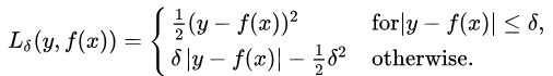
3. Huber Loss, Smooth Mean Absolute Error
Compared to squared error loss, Huber loss is less sensitive to outliers in the data, and it is also differentiable at 0. When the error is small, it becomes the quadratic error; how small the error must be to become a quadratic function depends on the hyperparameter 𝛿 (delta), which is adjustable.
When the hyperparameter 𝛿 ~ 0, the Huber loss method approaches MAE; when the hyperparameter 𝛿 ~ ∞, the Huber loss method approaches MSE.

The Huber curve is shown below, where the curves of different colors represent different hyperparameters (with true values equal to 0).
Choosing the hyperparameter 𝛿 is crucial because it determines which outliers you are willing to consider. Residuals greater than 𝛿 are minimized using L1, as L1 is less sensitive to larger outliers, while residuals less than 𝛿 are minimized using L2.
Why use Huber Loss?
A major issue with training neural networks using MAE is that its gradient is a relatively large constant, which can lead to missing the minimum when using gradient descent training. For MSE, the gradient decreases as the loss function approaches its minimum, making it easier to find the minimum.
Huber loss is helpful in this case because it reduces the gradient near the minimum and is more robust than MSE. Therefore, Huber loss combines the advantages of both MSE and MAE; however, the issue with Huber loss is that we may need to tune the hyperparameter 𝛿, which is an iterative process.
4. Log-Cosh Loss
Log-Cosh is another function used in regression tasks. It is smoother than L2, and Log-Cosh is the logarithm of the hyperbolic cosine of the prediction error.

The Log-Cosh loss function curve with respect to the predicted values (with true values equal to 0):
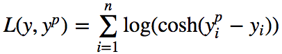
Advantages: When x is small, log(cosh(x)) approximates (x**2)/2; when x is large, it approximates abs(x) – log(2). This means that “logcosh” works similarly to MSE but is not affected by occasional outliers. It has all the advantages of Huber loss and is differentiable in any case.
Why do we need second derivatives?
Many ML model implementations (like XGBoost) use Newton’s method to find optimal values, which is why second-order derivatives (Hessian) are used. For ML frameworks like XGBoost, twice differentiable functions are more popular.
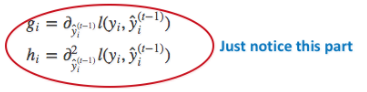
The objective function of xgboost:
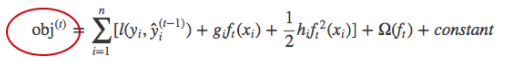
Where g_i and h_i are the first and second derivatives of the loss function l, respectively:
However, the logcosh loss is not perfect; when the predicted values deviate greatly from the true values, the gradient and second derivative are constants, which do not meet the splitting conditions of xgboost.
The Python code for Huber and Log-Cosh loss functions:
# huber loss
def huber(true, pred, delta):
    loss = np.where(np.abs(true-pred) < delta , 0.5*((true-pred)**2), delta*np.abs(true - pred) - 0.5*(delta**2))
    return np.sum(loss)

# log cosh loss
def logcosh(true, pred):
    loss = np.log(np.cosh(pred - true))
    return np.sum(loss)
5. Quantile Loss
In most real-world prediction problems, we are often interested in the uncertainty of predictions. Understanding the range of predictions (rather than just point estimates) can greatly improve the decision-making process for many business problems.
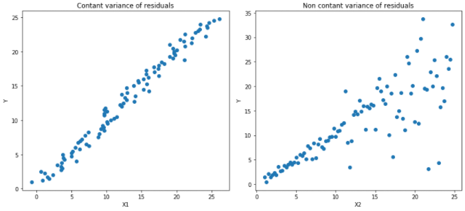
When we want to predict an interval rather than just a point, the quantile loss function is useful. The prediction interval of least squares regression is based on the assumption that the residuals (y-y_hat) have constant variance between the values of the independent variables.
We cannot trust a linear regression model that violates this assumption, nor can we abandon the idea of fitting a linear regression model as a baseline, as using non-linear functions or tree-based models is not necessarily better. This is where quantile loss and quantile regression come into play, providing reasonable prediction intervals for the residuals based on quantile loss, even when the variance of the residuals is not constant or not normally distributed.
Let’s take an example to better understand why quantile loss-based regression performs well in heteroscedastic data.
Quantile Regression vs Ordinary Least Squares Regression
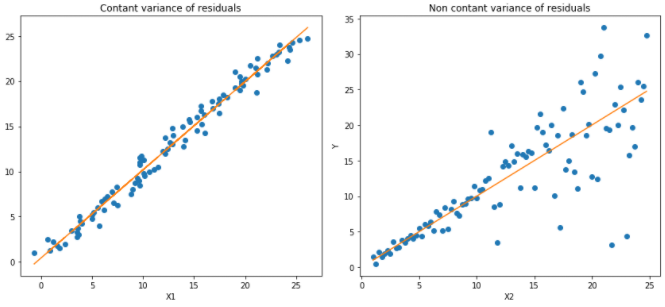
In the two types of data shown in the figure below, the left graph represents homoscedastic data, while the right graph represents heteroscedastic data:
The results of linear regression using least squares method:
Quantile regression for quantiles 0.05 and 0.95:
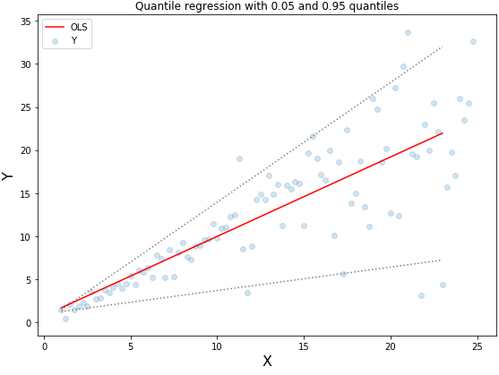
The dashed lines represent the regression based on quantile loss for 0.05 and 0.95 quantiles.
Understanding the Quantile Loss Function
Quantile regression estimates the conditional quantile of the response variable given the predictor variables. The quantile loss is essentially an extension of MAE, and when the quantile is 0.5, it is MAE.
The idea is to choose the quantile value based on how much weight we want to give to positive or negative errors, with the loss function giving different penalty weights to overestimated or underestimated predictions. For example, when setting the quantile γ = 0.25, the quantile loss function will penalize overestimated predictions more, keeping the predictions slightly below the median.
The quantile loss function:
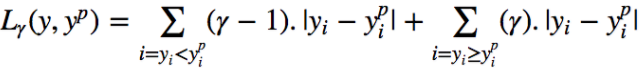
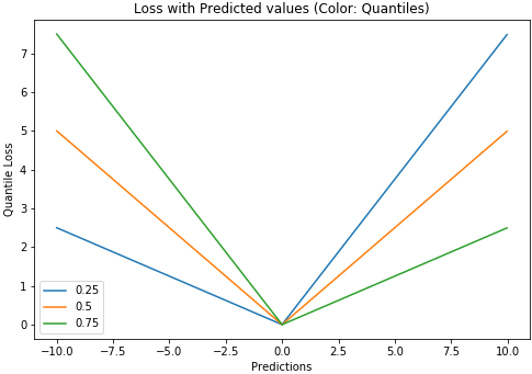
The value of quantile γ is between 0 and 1, and the relationship between the predicted values and the quantile regression loss function is shown in the figure below (with true values equal to 0).
We can also use this loss function to calculate prediction intervals for neural networks and tree-based models. Below is an example implementation for gradient-boosted tree regression using sklearn:
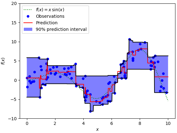
The upper limit of the 90% prediction interval in the figure above is the quantile equal to 0.95, and the lower limit is the quantile equal to 0.05.
Comparison of Four Regression Loss Functions
To compare the properties of the above loss functions, we simulate sinc function data and overlay two types of noise: Gaussian noise component ε ~ N(0, σ2) and impulse noise component ξ ~ Bern(p). To illustrate robustness, we added an impulse noise term. Below are the results of GBM fitting regression using different loss functions:
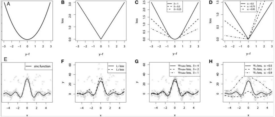
Where A represents the MSE loss equation, B represents the MAE loss equation, C represents the Huber loss equation, D represents the quantile loss equation, E represents the original sinc(x) data equation, F represents the fitting results of MSE loss and MAE loss, G represents the fitting results of Huber loss at different 𝛿 values, and H represents the fitting results of quantile loss.
Analyzing the regression results of different losses above, we can draw some conclusions:
1) The predictions with the MAE loss model are less affected by impulse noise, while the predictions with the MSE loss model are slightly biased due to noise.
2) The prediction results are not sensitive to the choice of hyperparameter for the Huber loss model.
3) Quantile loss can estimate the corresponding confidence level well.
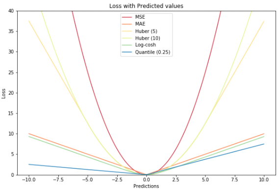
All regression loss functions plotted in one graph:
Feel free to scan the QR code to follow: