Produced by Big Data Digest

Compiled by: Hong Yingfei, Ning Jing

PyTorch, one of the deep learning framework libraries, is an open-source deep learning platform from Facebook that provides seamless transition from research prototypes to production deployment.

This article aims to introduce the basics of PyTorch, helping beginners write initial Python PyTorch code in 4 minutes.

All functional functions mentioned below can be found in the Chinese documentation for specific parameters and implementation details. Here is the link to the PyTorch Chinese documentation:

https://pytorch-cn.readthedocs.io/zh/latest/package_references/torch/

Preparation Before Coding

You need to install the Python package on your computer and import some scientific computing packages like numpy. Most importantly, don’t forget to import PyTorch. The running results below are obtained in Jupyter Notebook. Interested readers can download Anaconda, which comes with Jupyter Notebook. (Note: Anaconda supports multiple versions of Python in a virtual compilation environment, and Jupyter Notebook is a web-based compilation interface that divides code into cells, allowing real-time viewing of running results, making it very convenient!)

There are many tutorials online for software configuration and installation, which will not be elaborated here. Learning from books is always superficial; to truly understand, one must practice. Let’s directly enter the world of PyTorch and start coding!

Tensors

The Tensor class is an important basic data type in the neural network framework, which can be simply understood as a multi-dimensional matrix containing elements of a single data type. Tensors are connected through operations to form a computational graph.

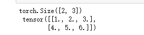
The following code example creates a 2×3 two-dimensional tensor x, specifying the data type as float:

import torch
# Tensors
x = torch.FloatTensor([[1, 2, 3], [4, 5, 6]])
print(x.size(), "\n", x)

Running result:

PyTorch includes many mathematical operations on tensors. In addition, it provides many utilities, such as efficient serialization of tensors and other arbitrary data types, as well as other useful utilities.

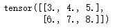
Below is an example of tensor addition/subtraction, where torch.ones(*sizes, out=None) → Tensor returns a tensor filled with 1, with the shape defined by the variable parameters sizes. In this example, the tensor created with values of 1 at corresponding positions is added to variable x, which is equivalent to adding 2 to each dimension of x. The code and running results are as follows:

# Add tensors
x.add_(torch.ones([2, 3]) + torch.ones([2, 3]))

Running result:

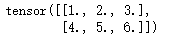
Similarly, PyTorch also supports subtraction operations, as shown in the example below, where 2 is subtracted from each dimension based on the running result above, restoring x to its original value.

# Subtract Tensor
x.sub_(torch.ones([2, 3]) * 2)

Running result:

Readers can refer to the Chinese link provided above for other PyTorch operations.

PyTorch and NumPy

Users can easily convert between PyTorch and NumPy.

Below is a simple example of converting np.matrix to PyTorch and changing the dimension to a single column:

# Numpy to torch tensors
import numpy as np
y = np.matrix([[2, 2], [2, 2], [2, 2]])
z = np.matrix([[2, 2], [2, 2], [2, 2]], dtype="int16")
x.short() @ torch.from_numpy(z)

Running result:

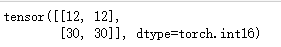
Here, @ is the overloaded operator for tensor multiplication, x is a 2×3 tensor with values [[1, 2, 3], [4, 5, 6]], multiplied by z converted to tensor, where z has a size of 3×2, resulting in a 2×2 tensor. (Similar to matrix multiplication, readers who do not understand the running results can refer to matrix multiplication operations)

In addition, PyTorch also supports reshaping tensor structures. Below is an example of reshaping tensor x into a 1×6 one-dimensional tensor, similar to the reshape function in NumPy.

# Reshape tensors (similar to np.reshape)
x.view(1, 6)

Running result:

GitHub repo outlines the conversion from PyTorch to NumPy, link as follows:

https://github.com/wkentaro/pytorch-for-numpy-users

CPU and GPUs

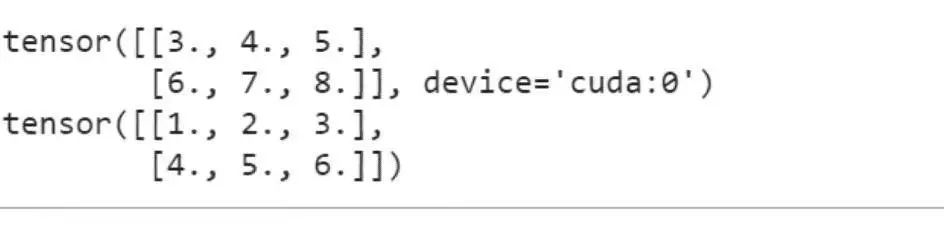
PyTorch allows variables to dynamically change devices using the torch.cuda.device context manager. Below is an example code:

# Move variables and copies across computer devices
x = torch.FloatTensor([[1, 2, 3], [4, 5, 6]])
y = np.matrix([[2, 2, 2], [2, 2, 2]], dtype="float32")

if(torch.cuda.is_available()):
    x = x.cuda();
    y = torch.from_numpy(y).cuda()
    z = x + y
print(z)
print(x.cpu())

Running result:

PyTorch Variables

Variables are just a thin layer wrapping tensors, supporting almost all APIs defined by tensors. Variables are cleverly defined as part of the automatic differentiation package. They provide classes and functions for implementing automatic differentiation of any scalar value function.

Below is a simple example of using PyTorch variables, where the result of multiplying v1 and v2 is assigned to v3. The attribute requires_grad inside defaults to False. If a node’s requires_grad is set to True, then all dependent nodes’ requires_grad will also be True, mainly used for gradient calculation.

# Variable (part of autograd package)
# Variable (graph nodes) are thin wrappers around tensors and have dependency knowledge
# Variable enable backpropagation of gradients and automatic differentiations
# Variable are set a 'volatile' flag during inference

from torch.autograd import Variable
v1 = Variable(torch.tensor([1., 2., 3.]), requires_grad=False)
v2 = Variable(torch.tensor([4., 5., 6.]), requires_grad=True)
v3 = v1 * v2

v3.data.numpy()

Running result:

# Variables remember what created them
v3.grad_fn

Running result:

Back Propagation

The backpropagation algorithm is used to compute the loss gradient with respect to input weights and biases to update the weights in the next optimization iteration and ultimately reduce the loss. PyTorch is very intelligent in defining the backward method for variables to perform backpropagation.

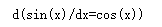
Below is a simple method for calculating backpropagation, taking the example of sin(x) to compute the difference:

# Backpropagation with example of sin(x)
x = Variable(torch.Tensor(np.array([0., 1., 1.5, 2.]) * np.pi), requires_grad=True)
y = torch.sin(x)
x.grad.backward(torch.Tensor([1., 1., 1., 1]))

# Check gradient is indeed cos(x)
if ((x.grad.data.int().numpy() == torch.cos(x).data.int().numpy()).all()):
    print("d(sin(x)/dx=cos(x))")

Running result:

For variables and gradient calculations in PyTorch, refer to the article below:

https://zhuanlan.zhihu.com/p/29904755

SLR: Simple Linear Regression

Now that we understand the basics, we can start using PyTorch to solve simple machine learning problems—simple linear regression. We will complete this in 4 simple steps:

Step One

In Step 1, we create a synthetic dataset generated by the equation y = wx + b and inject random errors. Please refer to the example below:

# Simple Linear Regression
# Fit a line to the data. Y = w.x + b
# Deterministic behavior
np.random.seed(0)
torch.manual_seed(0)
# Step 1: Dataset
w = 2;
b = 3
x = np.linspace(0, 10, 100)
y = w * x + b + np.random.randn(100) * 2
x = x.reshape(-1, 1)
y = y.reshape(-1, 1)

In Step 2, we define a simple class LinearRegressionModel using the forward function, utilizing torch.nn.Linear to define the constructor for linear transformation on input data:

# Step 2: Model
class LinearRegressionModel(torch.nn.Module):
    def __init__(self, in_dimn, out_dimn):
        super(LinearRegressionModel, self).__init__()
        self.model = torch.nn.Linear(in_dimn, out_dimn)

    def forward(self, x):
        y_pred = self.model(x);
        return y_pred;
model = LinearRegressionModel(in_dimn=1, out_dimn=1)

Reference for torch.nn.Linear:

https://pytorch.org/docs/stable/_modules/torch/nn/modules/linear.html

Step Three

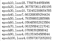
Next: use MSELoss as the cost function and SGD as the optimizer to train the model.

# Step 3: Training
cost = torch.nn.MSELoss()
optimizer = torch.optim.SGD(model.parameters(), lr=0.01, momentum=0.9)
inputs = Variable(torch.from_numpy(x.astype("float32")))
outputs = Variable(torch.from_numpy(y.astype("float32")))

for epoch in range(100):
    # 3.1 forward pass:
    y_pred = model(inputs)
    # 3.2 compute loss
    loss = cost(y_pred, outputs)
    # 3.3 backward pass
    optimizer.zero_grad();
    loss.backward()
    optimizer.step()
    if ((epoch + 1) % 10 == 0):
        print("epoch{}, loss{}".format(epoch + 1, loss.data))

Running result:

Reference for MSELoss:

https://pytorch.org/docs/stable/_modules/torch/nn/modules/loss.html

Reference for SGD:

https://pytorch.org/docs/stable/_modules/torch/optim/sgd.html

Step Four

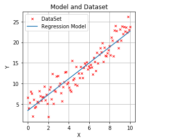
Now that training is complete, let’s visually check our model:

# Step 4: Display model and confirm
import matplotlib.pyplot as plt
plt.figure(figsize=(4, 4))
plt.title("Model and Dataset")
plt.xlabel("X");
plt.ylabel("Y")
plt.grid()
plt.plot(x, y, "ro", label="DataSet", marker="x", markersize=4)
plt.plot(x, model.model.weight.item() * x + model.model.bias.item(), label="Regression Model")
plt.legend();
plt.show()

Running result:

You have now completed the coding of your first linear regression example in PyTorch. For readers who wish to further their knowledge, you can refer to the official PyTorch documentation link to complete most coding applications.

Related links:

https://medium.com/towards-artificial-intelligence/pytorch-in-2-minutes-9e18875990fd