2D Path Planning Using CNN

Convolutional Neural Networks (CNN) are popular models for tasks such as image classification, segmentation, and object detection. This article applies CNN to solve simple 2D path planning problems using Python, PyTorch, NumPy, and OpenCV.

Task

Simply put, given a grid map, 2D path planning is about finding the shortest path from a given starting point to the desired target location (goal). Robotics is one of the main fields where path planning is crucial. Algorithms such as A*, D*, and D* lite and their related variants were developed to solve such problems. Nowadays, reinforcement learning is widely used to address this issue. This article will attempt to solve a simple path planning instance using only convolutional neural networks.

Dataset

Our main problem is (as always in machine learning) where to find the data. Although there is no ready-made dataset available, we can create our own path planning dataset by generating random 2D maps. The process of creating maps is very simple:

Start with a 100×100 pixel square empty matrix M.

For each element (pixel) in the matrix, draw a random number r uniformly from 0 to 1. If r > diff, set that pixel to 1; otherwise, set it to 0. Here, diff is a parameter that indicates the probability of a pixel becoming an obstacle (i.e., an impassable location), which is proportional to the difficulty of finding a viable path on that map.

Then we can use morphology to achieve a more realistic blocky effect similar to actual occupancy grid maps. By changing the size of the morphological structuring element and the diff parameter, we can generate maps with different difficulty levels.

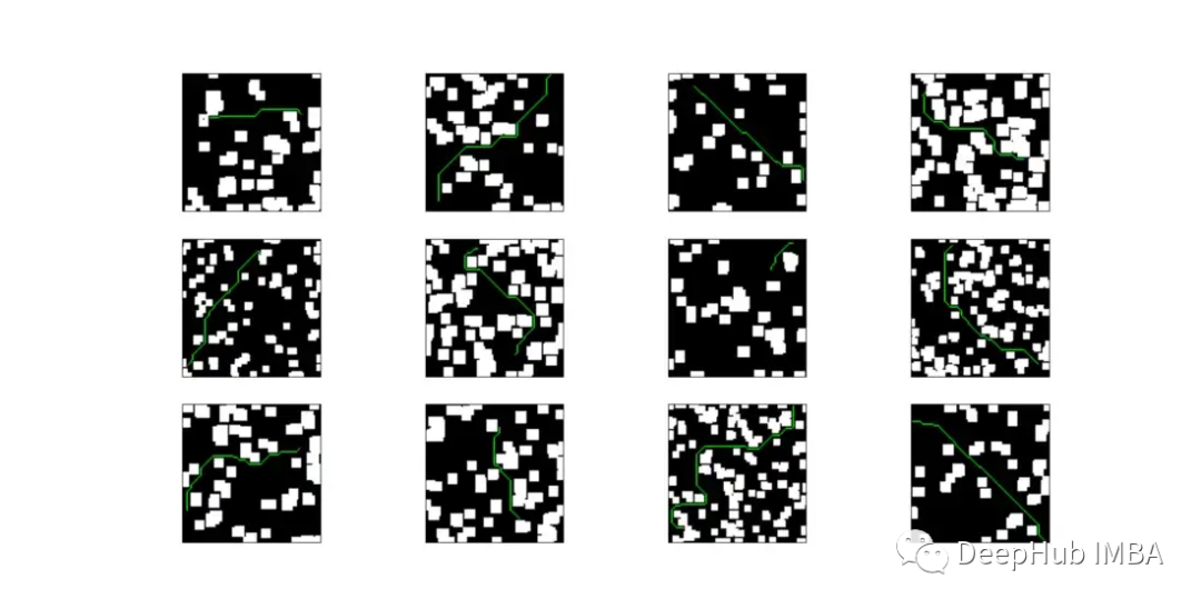
For each map, we need to choose 2 different locations: the starting point (s) and the goal point (g). This selection is also random, but this time we must ensure that the Euclidean distance between s and g is greater than a given threshold (to make the instance challenging).

Finally, we need to find the shortest path from s to g. This is the objective of our training. We can directly use the popular D* lite algorithm for this.

The dataset we generated contains approximately 230k samples (170k for training, 50k for testing, and 15k for validation). The volume of data is large, so I used the Boost C++ library to rewrite the custom D* lite as a Python extension module. Using this module, we can generate over 10k samples/hour, while using a pure Python implementation, the rate is about 1k samples/hour (i7–6500U 8GB RAM). The code for the custom D* lite implementation will be provided at the end of this article.

Then we perform some simple checks on the data, such as deleting maps with very high cosine similarity or where the starting and ending coordinates are too close. The data and code will also be provided at the end of this article.

Model Architecture

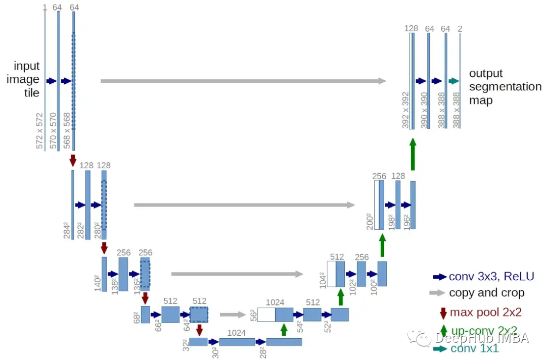
The model is a classic encoder-decoder architecture, consisting of 20 convolutional layers divided into 3 convolutional blocks (encoding part), followed by another 3 transposed convolutional blocks (decoding part). Each block consists of 3 3×3 convolutional layers, with BN and ReLU activation between each layer. Finally, there are 2 additional conv layers plus the output layer. The goal of the encoder is to find the relevant representation after compressing the input. The decoder part will attempt to reconstruct the same input mapping, but this time the useful information embedded should help find the best path from s to g.

The input to the network is:

map: a [n, 3, 100, 100] tensor representing the occupancy grid map. n is the batch size. Here, the number of channels is 3 instead of just 1. More details will be provided later.

• start: a [n, 2] tensor containing the coordinates of the starting point s in each map

• goal: a [n, 2] tensor containing the coordinates of the target point g in each map

The output layer of the network applies the sigmoid function, effectively providing a “score map” where the value of each item is between 0 and 1, proportional to the probability of being part of the shortest path from s to g. The path can then be reconstructed by starting from s and iteratively selecting the highest-scoring point in the current 8-neighborhood. Once a point with the same coordinates as g is found, the process ends. To improve efficiency, I used a bidirectional search algorithm for this.

Between the encoder and decoder blocks of the model, I also inserted 2 skip connections. The model is now very similar to the U-Net architecture. Skip connections inject the output of a given hidden layer into deeper layers of the network. The details we care about in our task are the exact locations of s and g, as well as all the obstacles we must avoid in the trajectory. Thus, adding skip connections greatly improves the performance.

Training

The model was trained for about 15 hours or 23 epochs on Google Colab. The loss function used was Mean Squared Error (MSE). There might be better choices than MSE, but I stuck with it because it is simple and easy to use.

The learning rate was initially set to 0.001 using the CosineAnnealingWithWarmRestarts scheduler (slightly modified to reduce the maximum learning rate after each restart). The batch size was set to 160.

I tried to apply Gaussian blur to the input map and a small dropout in the first convolutional layer. These techniques did not yield any relevant effects, so I ultimately abandoned them.

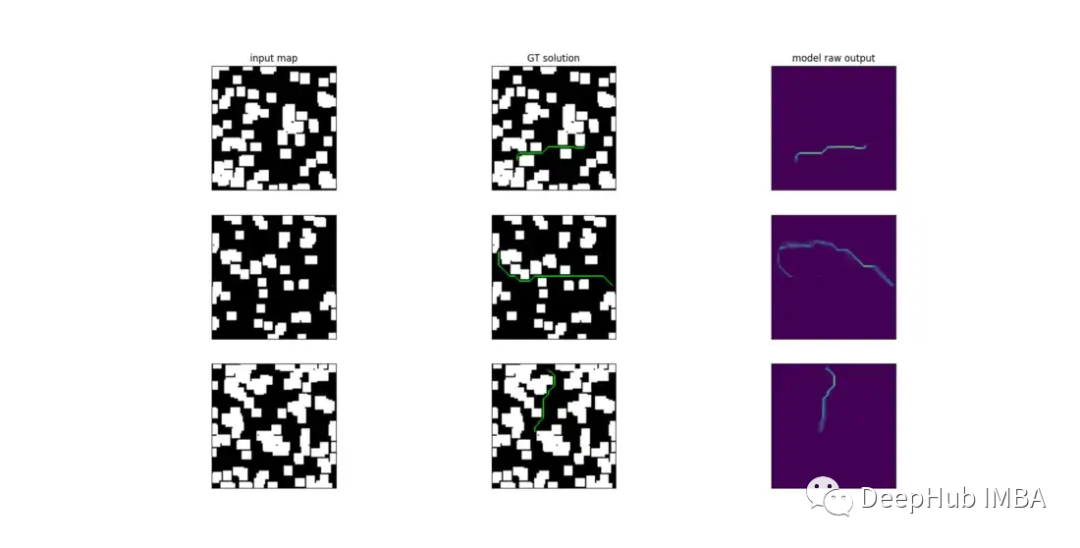
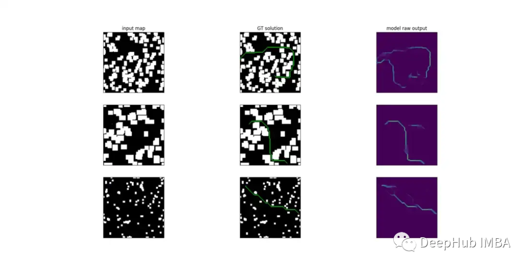
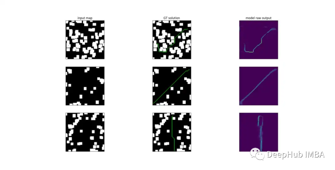
Below is a visualization of the original output of the model after training.

Some Issues with Convolution

Initially, the input was a tensor shaped [n, 1, 100, 100] (plus the starting and goal positions). However, I could not obtain any satisfactory results. The reconstructed path was just a random trajectory completely deviating from the target position and passing through obstacles.

A key feature of convolution operators is that they are position invariant. What convolution filters actually learn is a specific pixel pattern that appears repeatedly in the data distribution on which they are trained. For example, the pattern below can represent corners or vertical edges.

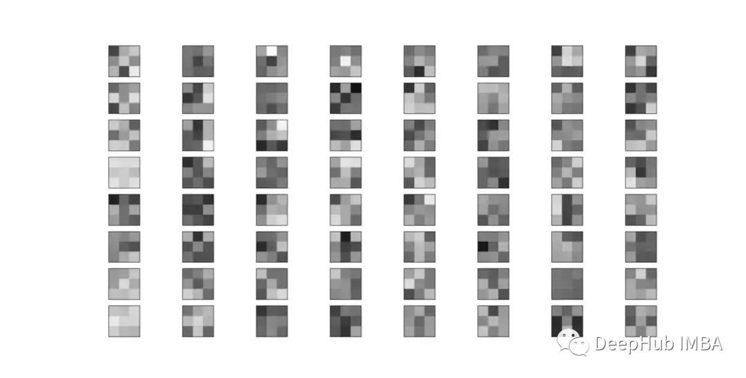
No matter what pattern the filter learns, the key issue is that it learns to recognize it independently of its position in the image. For tasks like image classification, this is undoubtedly an ideal feature since the patterns representing the target class may appear anywhere in the image. But in our case, the position is crucial! We need this network to be very clear about where the trajectory starts and ends.

Positional Encoding

Positional encoding is a technique that injects information about the position of data by embedding it (usually simply and) into the data itself. It is often applied in Natural Language Processing (NLP) to make the model aware of the position of words in a sentence. I thought something like this would also help our task.

I experimented with adding such positional encoding to the input occupancy map, but the results were not good. This might be because adding information about every possible position on the map contradicts the position invariance of convolution, making the filters useless.

So here, based on observations of path planning, we are not interested in absolute positions, but only in relative ranges. In other words, we care about the position of each cell in the occupancy grid relative to the starting point s and the goal point g. For example, for a cell at coordinates (x, y). I don’t really care if (x, y) equals (45,89) or (0,5). What we care about is that (x, y) is 34 cells away from s and 15 cells away from g.

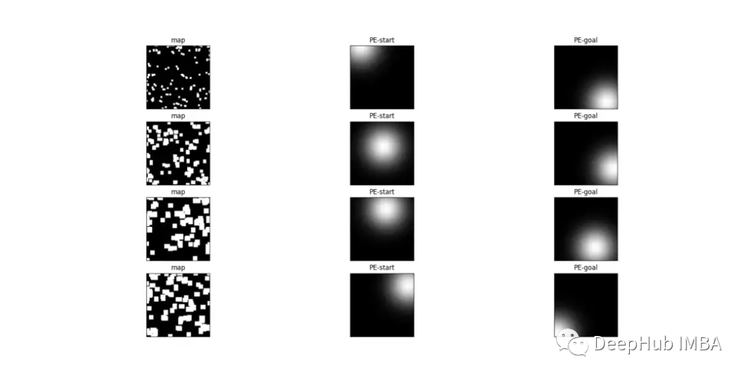
Thus, I created 2 additional channels for each occupancy grid map, now shaped [3,100,100]. The first channel is the image. The second channel represents a positional encoding that assigns a value to each pixel relative to the starting position. The third channel assigns a value relative to the ending position. This encoding is achieved by creating 2 feature maps from 2D Gaussian functions centered at s and g, respectively. Sigma is chosen to be one-fifth of the kernel size (usually in Gaussian filters). In our case, it is 20, and the map size is 100.

While injecting useful information about the expected starting and ending positions of the trajectory, we also partially preserve consistency with the invariance of the filter’s position. The learnable patterns now only depend on the distance relative to the given points, rather than every possible position on the map. Two equal patterns at the same distance from s or g will now trigger the same filter activation. This little trick proved to be very effective in converging training.

Results and Conclusion

The trained model was tested on over 51103 samples.

95% of the total test samples were able to provide solutions using bidirectional search. That is, the algorithm can find a path from s to g in 48556 samples using the score map provided by the model, while for the remaining 2547 samples, no path could be found.

87% of the total test samples provided valid solutions. That is, the trajectory from s to g did not cross any obstacles (this value does not consider the obstacle edge constraint of 1 cell).

On valid samples, the average error between the real path and the solution provided by the model is 33 cells. Considering the map is 100×100 cells, this is quite high. The error ranges from a minimum of 0 (i.e., the real path was “perfectly” reconstructed in 2491 samples) to a maximum of… 745 cells (there are definitely some issues here).

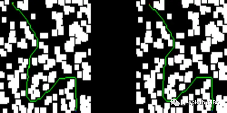
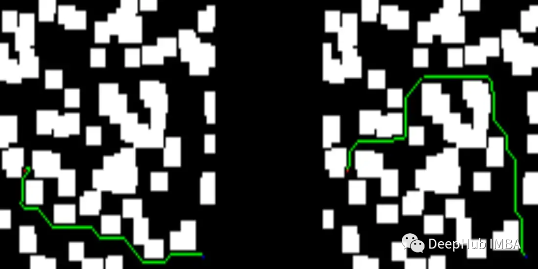
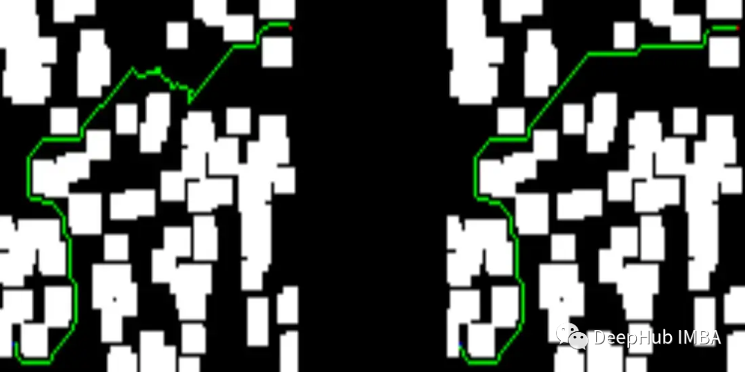
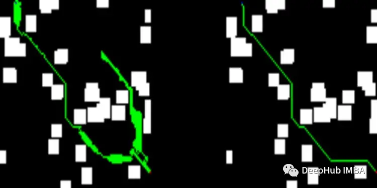
Below you can see some results from our test set. The left side of the image describes the solution provided by the trained network, while the right side shows the solution from the D* lite algorithm.

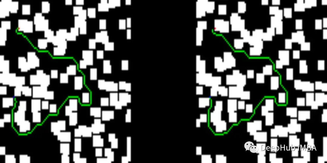
The solution provided by our network is shorter than that given by D* lite:

Below are some error images:

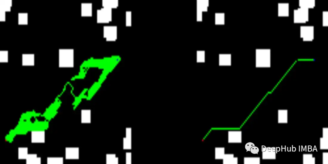
It seems that the receptive field is not large enough, so no edges were found within the area of the receptive field; this may need to be improved in the model.

Finally, this work is far from state-of-the-art results, and if you are interested, you can continue to improve it.