Reprinted from Algorithms and the Beauty of Mathematics
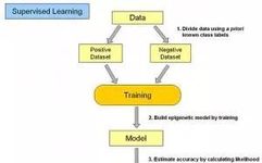
1. Supervised Learning:
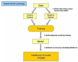
In supervised learning, the input data is referred to as “training data”, and each set of training data has a clear label or result, such as “spam” or “non-spam” in a spam detection system, or the digits “1”, “2”, “3”, “4”, etc. in handwritten digit recognition. When establishing a predictive model, supervised learning creates a learning process that compares the predicted results with the actual results of the “training data”, continuously adjusting the predictive model until the model’s predictions reach an expected accuracy.Common applications of supervised learning include classification and regression problems.Common algorithms include Logistic Regression and Back Propagation Neural Network.
2. Unsupervised Learning:
In unsupervised learning, the data is not specifically labeled, and the learning model is used to infer some inherent structure of the data.Common application scenarios include learning association rules and clustering.Common algorithms include Apriori and k-Means.
3. Semi-Supervised Learning:
In this learning approach, some input data is labeled while some is not. This learning model can be used for prediction, but the model first needs to learn the inherent structure of the data to organize the data reasonably for prediction. Application scenarios include classification and regression, and algorithms include extensions of common supervised learning algorithms that first attempt to model unlabeled data, and then predict labeled data based on that. Examples include Graph Inference Algorithms and Laplacian SVM.
4. Reinforcement Learning:
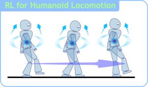
In this learning mode, input data serves as feedback to the model. Unlike supervised models where input data is merely a way to check the correctness of the model, in reinforcement learning, input data directly feeds back to the model, which must adjust immediately. Common application scenarios include dynamic systems and robot control.Common algorithms include Q-Learning and Temporal Difference Learning.
In the context of enterprise data applications, the most commonly used models are likely those of supervised and unsupervised learning. In fields like image recognition, where there is a large amount of unlabeled data and a small amount of labeled data, semi-supervised learning is currently a hot topic. Reinforcement learning is more often applied in robot control and other fields requiring system control.
5. Algorithm Similarity
Based on the similarity of the functions and forms of algorithms, we can classify algorithms, for example, tree-based algorithms, neural network-based algorithms, etc. Of course, the scope of machine learning is vast, and some algorithms are difficult to clearly categorize into one class. For some classifications, algorithms of the same category can address different types of problems.Here, we will try to classify commonly used algorithms in the most understandable way.
6. Regression Algorithms:
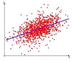
Regression algorithms attempt to explore the relationships between variables by measuring errors. Regression algorithms are powerful tools in statistical machine learning.In the field of machine learning, when people mention regression, it can sometimes refer to a type of problem or a type of algorithm, which can often confuse beginners. Common regression algorithms include: Ordinary Least Squares, Logistic Regression, Stepwise Regression, Multivariate Adaptive Regression Splines, and Locally Estimated Scatterplot Smoothing.
7. Instance-Based Algorithms
Instance-based algorithms are often used to model decision problems. These models typically select a batch of sample data and then compare new data with sample data based on certain similarities. This approach seeks the best match. Therefore, instance-based algorithms are often referred to as “winner-takes-all” learning or “memory-based learning”. Common algorithms include k-Nearest Neighbor (KNN), Learning Vector Quantization (LVQ), and Self-Organizing Map (SOM).
8. Regularization Methods
Regularization methods are extensions of other algorithms (usually regression algorithms), adjusting algorithms based on their complexity. Regularization methods typically reward simpler models while penalizing complex algorithms.Common algorithms include: Ridge Regression, Least Absolute Shrinkage and Selection Operator (LASSO), and Elastic Net.
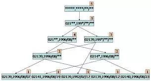
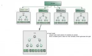
9. Decision Tree Learning
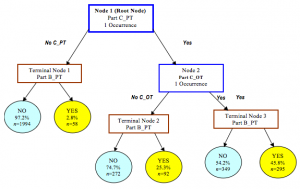
Decision tree algorithms establish decision models using a tree structure based on the attributes of the data. Decision tree models are often used to solve classification and regression problems. Common algorithms include: Classification And Regression Tree (CART), ID3 (Iterative Dichotomiser 3), C4.5, Chi-squared Automatic Interaction Detection (CHAID), Decision Stump, Random Forest, Multivariate Adaptive Regression Splines (MARS), and Gradient Boosting Machine (GBM).
10. Bayesian Methods
Bayesian methods are a class of algorithms based on Bayes’ theorem, primarily used to solve classification and regression problems. Common algorithms include: Naive Bayes, Averaged One-Dependence Estimators (AODE), and Bayesian Belief Network (BBN).
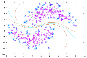
11. Kernel-Based Algorithms
The most famous kernel-based algorithm is the Support Vector Machine (SVM). Kernel-based algorithms map input data to a high-dimensional vector space, where some classification or regression problems can be solved more easily. Common kernel-based algorithms include: Support Vector Machine (SVM), Radial Basis Function (RBF), and Linear Discriminant Analysis (LDA).
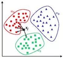
12. Clustering Algorithms
Clustering, like regression, sometimes describes a class of problems and sometimes describes a class of algorithms. Clustering algorithms usually merge input data either by centroids or hierarchically. All clustering algorithms attempt to find the inherent structure of the data in order to classify the data based on the greatest commonality.Common clustering algorithms include k-Means and Expectation Maximization (EM).
13. Association Rule Learning
Association rule learning seeks to find rules that best explain the relationships between data variables, in order to identify useful association rules in large multi-dimensional data sets. Common algorithms include Apriori and Eclat.
14. Artificial Neural Networks
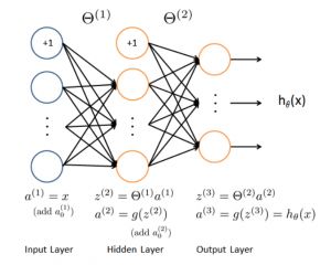
Artificial neural network algorithms simulate biological neural networks and are a class of pattern matching algorithms. They are typically used to solve classification and regression problems. Artificial neural networks represent a vast branch of machine learning, with hundreds of different algorithms. (Deep learning is one such algorithm that we will discuss separately). Important artificial neural network algorithms include: Perceptron Neural Network, Back Propagation, Hopfield Network, Self-Organizing Map (SOM), and Learning Vector Quantization (LVQ).
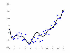
15. Deep Learning
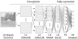
Deep learning algorithms are developments of artificial neural networks. They have gained much attention recently, especially since Baidu has also started focusing on deep learning, which has attracted considerable attention domestically. In an era where computing power has become increasingly inexpensive, deep learning attempts to build much larger and more complex neural networks. Many deep learning algorithms are semi-supervised learning algorithms used to handle large data sets with a small amount of unlabeled data. Common deep learning algorithms include: Restricted Boltzmann Machine (RBM), Deep Belief Networks (DBN), Convolutional Networks, and Stacked Auto-encoders.
16. Dimensionality Reduction Algorithms
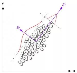
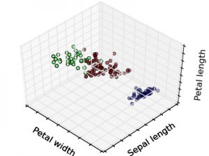
Like clustering algorithms, dimensionality reduction algorithms attempt to analyze the inherent structure of data, but they do so in an unsupervised learning manner, attempting to generalize or explain the data using less information.This class of algorithms can be used for visualizing high-dimensional data or simplifying data for supervised learning purposes.
Common algorithms include: Principal Component Analysis (PCA), Partial Least Square Regression (PLS), Sammon Mapping, Multi-Dimensional Scaling (MDS), and Projection Pursuit.
17. Ensemble Algorithms:
Ensemble algorithms train several relatively weak learning models independently on the same samples and then integrate the results to make overall predictions. The main difficulty of ensemble algorithms lies in selecting which independent weak learning models to integrate and how to combine the learning results.
This is a very powerful class of algorithms and is also very popular. Common algorithms include: Boosting, Bootstrapped Aggregation (Bagging), AdaBoost, Stacked Generalization (Blending), Gradient Boosting Machine (GBM), and Random Forest.
Common Advantages and Disadvantages of Machine Learning Algorithms:
Naive Bayes:
1. If the given feature vector lengths may vary, they need to be normalized to a common length vector (taking text classification as an example), for instance, if it is a sentence of words, the length corresponds to the total vocabulary length, with the corresponding position being the count of that word’s occurrences.
2. The calculation formula is as follows:
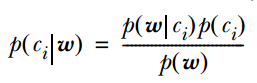
One of the conditional probabilities can be expanded through the naive Bayes conditional independence assumption. Note that  can be calculated, and based on the naive Bayes assumption,
  =
= , thus generally, there are two methods: one is to find the total occurrences of wj in the samples of class ci and divide by the total of that sample; the second method is to find the total occurrences of wj in the samples of class ci and divide by the total occurrences of all features in that sample.
3. If any item in  is 0, then the product of the joint probabilities may also be 0, meaning the numerator in formula 2 is 0. To avoid this phenomenon, generally, this item will be initialized to 1, and of course, to ensure equal probabilities, the denominator should be initialized to 2 (since there are 2 classes, add 2; if there are k classes, add k, a term known as Laplace smoothing, the reason for adding k to the denominator is to satisfy the total probability formula).
Advantages of Naive Bayes:Performs well on small-scale data, suitable for multi-class tasks, and suitable for incremental training.
Disadvantages:Very sensitive to the representation of input data.
Decision Trees:In decision trees, an important aspect is selecting an attribute for branching, so it is important to pay attention to the calculation formula for information gain and to understand it deeply.
The calculation formula for information entropy is as follows:
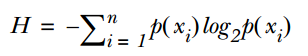
Where n represents the number of classification categories (for example, assuming a binary problem, n=2). Calculate the probabilities p1 and p2 of these 2 class samples appearing in the total samples, thus calculating the information entropy before selecting an attribute for branching.
Now selecting an attribute xi for branching, the branching rule is: if xi=vx, the sample is assigned to one branch of the tree; if not equal, it goes to the other branch. It is clear that the samples in the branch are likely to include 2 categories, calculating the entropies H1 and H2 of these 2 branches, the total information entropy after branching is H’=p1*H1+p2*H2, then the information gain ΔH=H-H’. Following the principle of information gain, test all attributes and choose the one with the maximum gain as the branching attribute for this time.
Advantages of decision trees:Simple computation, strong interpretability, suitable for handling samples with missing attribute values, and able to handle irrelevant features;
Disadvantages:Prone to overfitting (subsequently, random forests appeared to reduce the overfitting phenomenon).
Logistic Regression:Logistic is used for classification and is a type of linear classifier. Points to note include:
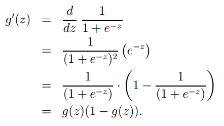
1. The logistic function expression is:
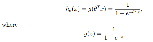
Its derivative form is:
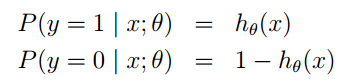
2. The logistic regression method mainly uses maximum likelihood estimation for learning, so the posterior probability of a single sample is:
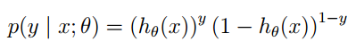
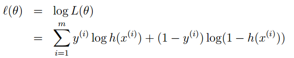
To the posterior probability of the entire sample:
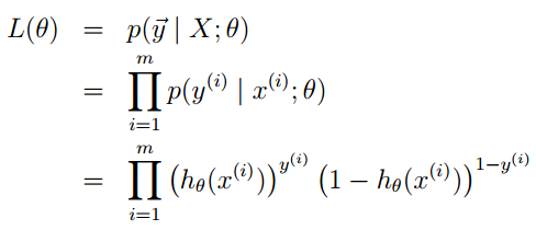
Where:
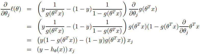
By simplifying through logarithms:
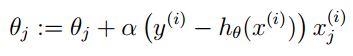
3. Its loss function is -l(θ), thus we need to minimize the loss function, which can be achieved using gradient descent. The gradient descent formula is:
Advantages of Logistic Regression:
1. Simple to implement
2. Very fast during classification with low computational resources;
Disadvantages:
1. Prone to underfitting, generally with low accuracy
2. Can only handle binary classification problems (the derived softmax can be used for multi-class), and must be linearly separable;
Linear Regression:
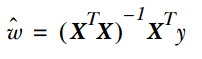
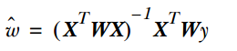
Linear regression is truly used for regression, unlike logistic regression which is used for classification. The basic idea is to optimize the error function in the form of least squares using gradient descent, and it can also use the normal equation to directly obtain the parameter solution, resulting in:
In LWLR (Locally Weighted Linear Regression), the parameter calculation expression is:
Because at this time, the optimization is:
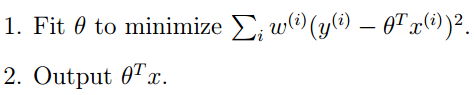
Thus, it can be seen that LWLR differs from LR, as LWLR is a non-parametric model since each regression calculation must traverse the training samples at least once.
Advantages of Linear Regression:Simple implementation, simple computation;
Disadvantages:Cannot fit non-linear data;
KNN Algorithm:KNN, or the k-Nearest Neighbors algorithm, primarily involves the following steps:
1. Calculate the distance between each sample point in the training and testing samples (common distance metrics include Euclidean distance, Mahalanobis distance, etc.);
2. Sort all the distance values obtained above;
3. Select the top k samples with the smallest distances;
4. Based on the labels of these k samples, perform voting to obtain the final classification category;
Choosing the best K value depends on the data. Generally, a larger K value can reduce the influence of noise, but it can make the boundaries between categories more ambiguous. A good K value can be obtained through various heuristic techniques, such as cross-validation.Additionally, the presence of noise and irrelevant feature vectors can decrease the accuracy of the KNN algorithm.
The nearest neighbor algorithm has strong consistency results. As the data approaches infinity, the algorithm guarantees that the error rate will not exceed twice the error rate of the Bayesian algorithm. For some good K values, KNN guarantees that the error rate will not exceed the Bayesian theoretical error rate.
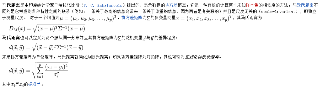
Note: The Mahalanobis distance must first provide the statistical properties of the sample set, such as mean vector, covariance matrix, etc. An introduction to the Mahalanobis distance is as follows:
KNN Algorithm Advantages:
1. Simple concept, mature theory, can be used for both classification and regression;
2. Can be used for non-linear classification;
3. Training time complexity is O(n);
4. High accuracy, no assumptions about the data, insensitive to outliers;
Disadvantages:
1. High computational cost;
2. Sample imbalance issue (i.e., some categories have many samples while others have very few);
3. Requires a large amount of memory;
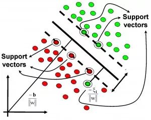
SVM:
It is important to learn how to use libsvm and some parameter adjustment experiences, and to clarify some ideas of the SVM algorithm:
1. The optimal classification surface in SVM maximizes the geometric margin for all samples (why choose the maximum margin classifier? Please explain from a mathematical perspective. This question was asked during an interview for a deep learning position at NetEase. The answer is that the geometric margin is related to the error rate of the samples: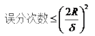 , where the denominator is the distance from the sample to the classification margin, and R in the numerator is the longest vector value among all samples), that is:
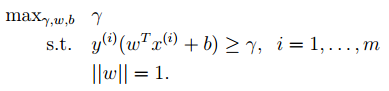
After a series of derivations, we can optimize the following original objective:

2. Now let’s take a look at Lagrange theory:
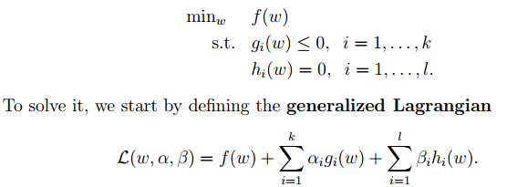
We can convert the optimization objective in 1 to the form of Lagrange (through various dual optimizations, KKD conditions), and the final objective function is:
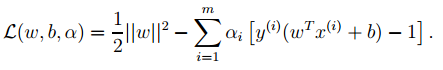
We only need to minimize the above objective function, where α is the Lagrange coefficient of the inequality constraints in the original optimization problem.
3. Taking the derivatives of w and b from the final expression in 2 gives:
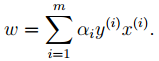
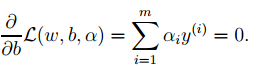
From the first expression above, we can see that if we optimize α, we can directly determine w, i.e., the model parameters are fixed. The second expression can serve as a constraint for subsequent optimization.
4. By applying dual optimization theory to the last objective function in 2, we can convert it to the optimization of the following objective function:
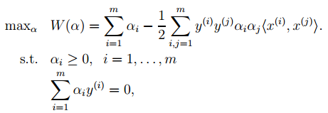
This function can be solved for α using common optimization methods, and subsequently, w and b can be determined.
5. Theoretically, the simple theory of SVM should end here. However, it is worth adding that during prediction:
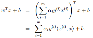
The angle brackets can be replaced with kernel functions, which is why SVM is often associated with kernel functions.
6. Finally, regarding the introduction of slack variables, the original optimization formula is:
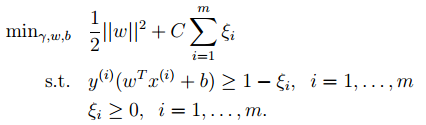
The corresponding dual optimization formula is:
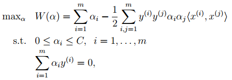
Compared to the previous one, the only difference is that α has an upper bound.
SVM Algorithm Advantages:
1. Can be used for linear/non-linear classification and also for regression;
2. Low generalization error;
3. Easy to interpret;
4. Low computational complexity;
Disadvantages:
1. Sensitive to the choice of parameters and kernel functions;
2. The original SVM is only particularly adept at handling binary classification problems;
Boosting:
Mainly taking Adaboost as an example, let’s first look at the flowchart of Adaboost:
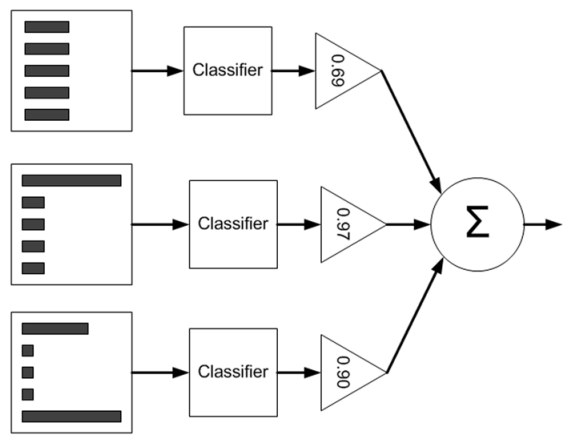
As seen in the diagram, during the training process we need to train multiple weak classifiers (3 in the diagram), each weak classifier is trained with samples of different weights (5 training samples in the diagram), and each weak classifier contributes differently to the final classification result, outputting through weighted averages, with the weights shown in the triangle in the diagram. So how are these weak classifiers and their corresponding weights trained?
Let’s illustrate with a simple example, assuming there are 5 training samples, each with a dimension of 2. When training the first classifier, the weights of the 5 samples are equal at 0.2. Note that the sample weights and the weights α corresponding to the final trained weak classifiers are different; the sample weights are only used during training, while α is used during both the training and testing processes.
Now assume the weak classifier is a simple decision tree with one node that selects one of the 2 attributes (assuming there are only 2 attributes) and computes the optimal value of that attribute for classification.
Here is a simple version of the training process for Adaboost:
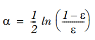
1. Train the first classifier with equal weights D for the samples. Through a weak classifier, obtain the predicted labels for these 5 samples (please refer to the example in the book, still from Machine Learning in Action) and compare with the true labels to find errors (i.e., mistakes). If a sample is misclassified, its corresponding error value is the weight of that sample, and if classified correctly, the error value is 0. Finally, sum the errors of the 5 samples, denoted as ε.
2. Use ε to calculate the weight α of the weak classifier, as follows:
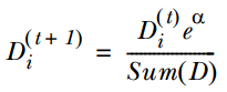
3. Using α to calculate the weights D of the samples for training the next weak classifier, if the corresponding sample is classified correctly, reduce that sample’s weight, the formula is:
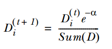
If the sample is misclassified, increase that sample’s weight, the formula is:
4. Repeat steps 1, 2, and 3 to continue training multiple classifiers, just with different D values.
The testing process is as follows:
Input a sample into each trained weak classifier, and each weak classifier corresponds to an output label, then that label is multiplied by its corresponding α, and finally, the sum is taken to determine the sign of the predicted label value.
Advantages of Boosting Algorithms:
1. Low generalization error;
2. Easy to implement, high classification accuracy, with few parameters to adjust;
3. Disadvantages:
4. Sensitive to outliers;
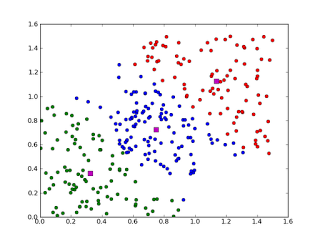
Clustering:
Based on clustering ideas, we can divide it into:
1. Partition-based clustering:
k-means, k-medoids (find a sample point to represent each category), CLARANS.
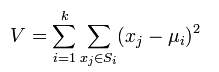
k-means minimizes the following expression:
Advantages of k-means algorithm:
(1) The k-means algorithm is a classic algorithm for solving clustering problems, simple and fast.
(2) For handling large datasets, the algorithm is relatively scalable and efficient, with a complexity of approximately O(nkt), where n is the number of all objects, k is the number of clusters, and t is the number of iterations. Typically, k << n. This algorithm usually converges locally.
(3) The algorithm attempts to find the k partitions that minimize the sum of squared errors. The clustering effect is better when the clusters are dense, spherical, or globular, and clearly distinguishable from each other.
Disadvantages:
(1) The k-means method can only be used when the average of clusters is defined, and it is not suitable for some categorical data attributes.
(2) Requires the user to specify the number of clusters k in advance.
(3) Sensitive to initial values; different initial values can lead to different clustering results.
(4) Not suitable for discovering clusters with non-convex shapes or clusters of significantly different sizes.
(5) Sensitive to