Introduction

This article reviews some cleverly designed and practical “plug-ins” for CNN networks. A “plug-in” should not alter the main structure of the network and can be easily embedded into mainstream networks to enhance feature extraction capabilities, achieving plug-and-play functionality. Many networks claim to offer plug-and-play solutions, but through my experience and research, I found that many plug-ins are impractical, non-generalizable, or even ineffective, leading to this compilation.

First, my understanding is: since it is a “plug-in”, it should enhance the performance while being easy to integrate and truly plug-and-play. The “plug-ins” discussed in this article can be seen in many SOTA networks. They are conscientious “plug-ins” worth promoting, truly capable of achieving plug-and-play functionality. In short, they are “plug-ins” that work. Many “plug-ins” are introduced to enhance CNN capabilities, such as translation, rotation, scaling, multi-scale feature extraction, receptive field enhancement, and spatial position perception.

List of Candidates: STN, ASPP, Non-local, SE, CBAM, DCNv1&v2, CoordConv, Ghost, BlurPool, RFB, ASFF

1 STN

From Paper: Spatial Transformer Networks

Paper Link: https://arxiv.org/pdf/1506.02025.pdf

Core Analysis:

In tasks like OCR, you will often see its presence. For CNN networks, we hope they possess invariance to object posture and position. That is, they can adapt to certain posture and position variations on the test set. Invariance or equivariance can effectively improve the model’s generalization ability. Although CNNs use sliding-window convolution operations, which have some degree of translational invariance, many studies have found that downsampling can destroy the network’s translational invariance. Therefore, it can be said that the network’s invariance capability is very weak, let alone invariance under rotation, scale, and lighting changes. Generally, we utilize data augmentation to achieve network “invariance”.

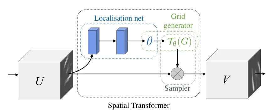
This article proposes the STN module, which explicitly embeds spatial transformations into the network, thereby enhancing the network’s invariance to rotation, translation, and scale. It can be understood as an “alignment” operation. The structure of STN is shown in the figure above, with each STN module consisting of a Localisation net, a Grid generator, and a Sampler. The Localisation net learns the parameters for spatial transformation, which are the six parameters in the above equation. The Grid generator is used for coordinate mapping. The Sampler is responsible for pixel sampling, utilizing bilinear interpolation.

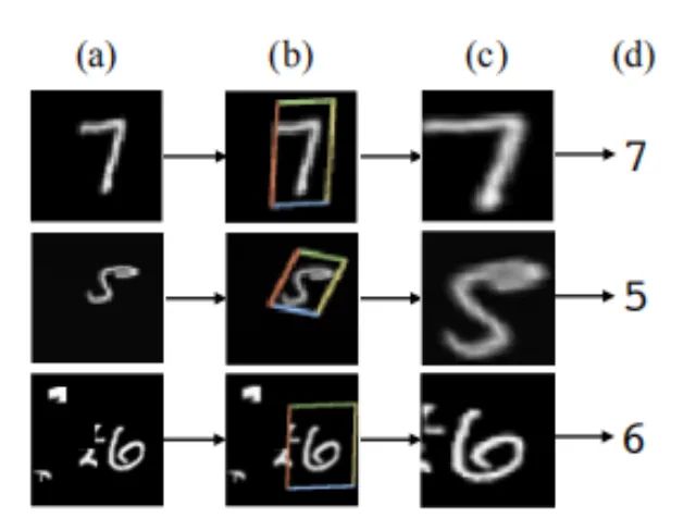
The significance of STN is that it can correct the original image into the desired ideal image for the network, and this process is performed in an unsupervised manner, meaning that the transformation parameters are learned spontaneously without the need for labeled information. This module is an independent module that can be inserted at any position in the CNN. It meets the requirements for this “plug-in” compilation.

Core Code:

class SpatialTransformer(nn.Module):
    def __init__(self, spatial_dims):
        super(SpatialTransformer, self).__init__()
        self._h, self._w = spatial_dims
        self.fc1 = nn.Linear(32*4*4, 1024) # Set according to your network parameters
        self.fc2 = nn.Linear(1024, 6)
    def forward(self, x):
        batch_images = x # Save a copy of the original data
        x = x.view(-1, 32*4*4)
        # Learn the 6 parameters using FC structure
        x = self.fc1(x)
        x = self.fc2(x)
        x = x.view(-1, 2, 3) # 2x3
        # Generate sampling points using affine_grid
        affine_grid_points = F.affine_grid(x, torch.Size((x.size(0), self._in_ch, self._h, self._w)))
        # Apply sampling points to the original data
        rois = F.grid_sample(batch_images, affine_grid_points)
        return rois, affine_grid_points

2 ASPP

Full Name of Plug-in: atrous spatial pyramid pooling

From Paper: DeepLab: Semantic Image Segmentation with Deep Convolutional Nets, Atrous Conv

Paper Link: https://arxiv.org/pdf/1606.00915.pdf

Core Analysis:

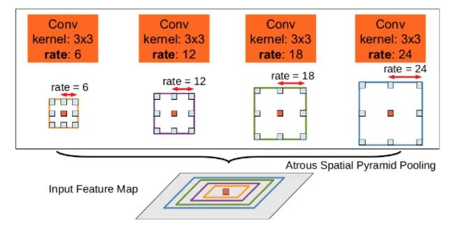
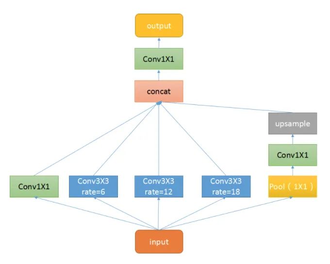
This plug-in is a spatial pyramid pooling module with dilated convolution, mainly aimed at enhancing the network’s receptive field and introducing multi-scale information. We know that for semantic segmentation networks, they typically face high-resolution images, which require our networks to have sufficient receptive fields to cover the target objects. CNN networks primarily rely on the stacking of convolutional layers and downsampling operations to achieve receptive fields. This module can control the receptive field size without changing the feature map size, which is beneficial for extracting multi-scale information. The rate controls the size of the receptive field; the larger the r, the larger the receptive field.

ASPP mainly consists of the following parts: 1. A global average pooling layer to obtain image-level features, followed by a 1X1 convolution, and then bilinearly interpolated to the original size; 2. A 1X1 convolution layer, along with three 3X3 dilated convolutions; 3. The five features at different scales are concatenated along the channel dimension and then sent into a 1X1 convolution for fusion output.

Core Code:

class ASPP(nn.Module):
    def __init__(self, in_channel=512, depth=256):
        super(ASPP,self).__init__()
        self.mean = nn.AdaptiveAvgPool2d((1, 1))
        self.conv = nn.Conv2d(in_channel, depth, 1, 1)
        self.atrous_block1 = nn.Conv2d(in_channel, depth, 1, 1)
        # Convolutions with different dilation rates
        self.atrous_block6 = nn.Conv2d(in_channel, depth, 3, 1, padding=6, dilation=6)
        self.atrous_block12 = nn.Conv2d(in_channel, depth, 3, 1, padding=12, dilation=12)
        self.atrous_block18 = nn.Conv2d(in_channel, depth, 3, 1, padding=18, dilation=18)
        self.conv_1x1_output = nn.Conv2d(depth * 5, depth, 1, 1)
    def forward(self, x):
        size = x.shape[2:]     # Pooling branch
        image_features = self.mean(x)
        image_features = self.conv(image_features)
        image_features = F.upsample(image_features, size=size, mode='bilinear')     # Convolutions with different dilation rates
        atrous_block1 = self.atrous_block1(x)
        atrous_block6 = self.atrous_block6(x)
        atrous_block12 = self.atrous_block12(x)
        atrous_block18 = self.atrous_block18(x)
        # Combine features from all scales
        x = torch.cat([image_features, atrous_block1, atrous_block6,atrous_block12, atrous_block18], dim=1)
        # Use 1X1 convolution to fuse features for output
        x = self.conv_1x1_output(x)
        return net

3 Non-local

From Paper: Non-local Neural Networks

Paper Link: https://arxiv.org/abs/1711.07971

Core Analysis:

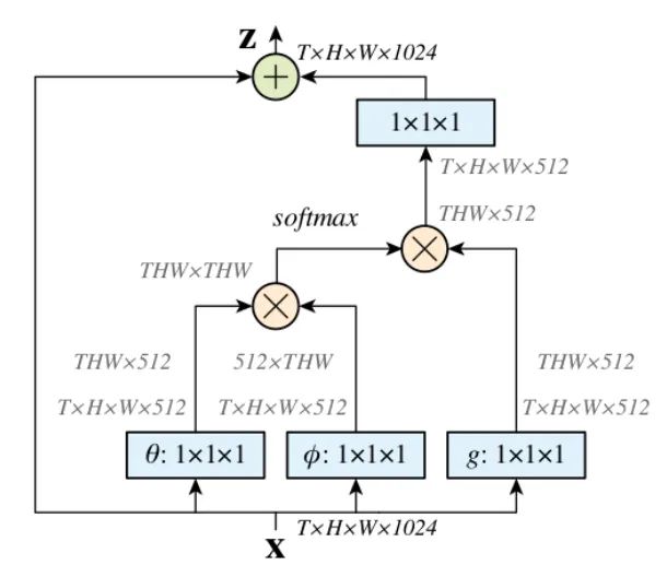
Non-Local is an attention mechanism and an easily integrated module. Local operations are primarily concerned with the receptive field, as seen in CNN’s convolution and pooling operations, where the size of the receptive field corresponds to the size of the convolution kernel. When we commonly stack 3X3 convolutional layers, they only consider local regions, performing local operations. In contrast, non-local operations can have a large receptive field, potentially covering global areas rather than just local regions. It captures long-range dependencies, establishing connections between pixels at a certain distance in the image through an attention mechanism. The attention mechanism generates a saliency map, where attention corresponds to salient areas that the network should focus on.

• First, perform a 1X1 convolution on the input feature map to reduce the channel count, obtaining features.
• Next, reshape the dimensions of the three features and perform matrix multiplication to obtain a covariance matrix-like result, which calculates the self-correlation of features, determining the relationship of each pixel in every frame to all pixels in other frames.
• Then, apply Softmax to the self-correlation features to obtain weights ranging from 0 to 1, which represent the self-attention coefficients.
• Finally, multiply the attention coefficients back onto the feature matrix g and add the residual from the original input feature map X for output.

Here’s a simple example for understanding: assuming g is (temporarily ignoring batch and channel dimensions):

g = torch.tensor([[1, 2],
                           [3, 4]).view(-1, 1).float()

and:

theta = torch.tensor([2, 4, 6, 8]).view(-1, 1)

and:

phi = torch.tensor([7, 5, 3, 1]).view(1, -1)

Then, the matrix multiplication is as follows:

tensor([[14., 10.,  6.,  2.],
                [28., 20., 12.,  4.],
                [42., 30., 18.,  6.],
                [56., 40., 24.,  8.]])

After applying softmax(dim=-1), we get:

tensor([[9.8168e-01, 1.7980e-02, 3.2932e-04, 6.0317e-06],
                [9.9966e-01, 3.3535e-04, 1.1250e-07, 3.7739e-11],
                [9.9999e-01, 6.1442e-06, 3.7751e-11, 2.3195e-16],
                [1.0000e+00, 1.1254e-07, 1.2664e-14, 1.4252e-21]])

With the attention applied, the overall values converge towards 1:

tensor([[1.0187, 1.0003],
                [1.0000, 1.0000]])

Core Code:

class NonLocal(nn.Module):
    def __init__(self, channel):
        super(NonLocalBlock, self).__init__()
        self.inter_channel = channel // 2
        self.conv_phi = nn.Conv2d(channel, self.inter_channel, 1, 1,0, False)
        self.conv_theta = nn.Conv2d(channel, self.inter_channel, 1, 1,0, False)
        self.conv_g = nn.Conv2d(channel, self.inter_channel, 1, 1, 0, False)
        self.softmax = nn.Softmax(dim=1)
        self.conv_mask = nn.Conv2d(self.inter_channel, channel, 1, 1, 0, False)
    def forward(self, x):
        # [N, C, H , W]
        b, c, h, w = x.size()
        # Get phi features, dimensions [N, C/2, H * W], preserving batch and channel dimensions, processed on HW
        x_phi = self.conv_phi(x).view(b, c, -1)
        # Get theta features, dimensions [N, H * W, C/2]
        x_theta = self.conv_theta(x).view(b, c, -1).permute(0, 2, 1).contiguous()
        # Get g features, dimensions [N, H * W, C/2]
        x_g = self.conv_g(x).view(b, c, -1).permute(0, 2, 1).contiguous()
        # Perform matrix multiplication between phi and theta, [N, H * W, H * W]
        mul_theta_phi = torch.matmul(x_theta, x_phi)
        # Softmax to bring values between 0 and 1
        mul_theta_phi = self.softmax(mul_theta_phi)
        # Multiply with g features, [N, H * W, C/2]
        mul_theta_phi_g = torch.matmul(mul_theta_phi, x_g)
        # [N, C/2, H, W]
        mul_theta_phi_g = mul_theta_phi_g.permute(0, 2, 1).contiguous().view(b, self.inter_channel, h, w)
        # 1X1 convolution to expand channel count
        mask = self.conv_mask(mul_theta_phi_g)
        out = mask + x # Residual connection
        return out

4 SE

From Paper: Squeeze-and-Excitation Networks

Paper Link: https://arxiv.org/pdf/1709.01507.pdf

Core Analysis:

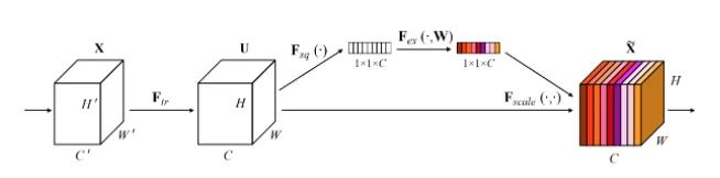
This is the championship work of the last ImageNet competition, and you can see its presence in many classic network structures, such as Mobilenet v3. It is essentially a channel attention mechanism. Due to feature compression and FC layers, the captured channel attention features contain global information. This article proposes a new structural unit – the “Squeeze-and-Excitation (SE)” module, which can adaptively adjust the feature response values of each channel, modeling the internal dependencies between channels. The steps are as follows:

• Squeeze: Compress features along the spatial dimension, turning each 2D feature channel into a single number, providing a global receptive field.

• Excitation: Each feature channel generates a weight representing the importance of that feature channel.

• Reweight: The weights produced by Excitation are viewed as the importance of each feature channel and are applied to each channel through multiplication.

Core Code:

class SE_Block(nn.Module):
    def __init__(self, ch_in, reduction=16):
        super(SE_Block, self).__init__()
        self.avg_pool = nn.AdaptiveAvgPool2d(1)  # Global adaptive pooling
        self.fc = nn.Sequential(
            nn.Linear(ch_in, ch_in // reduction, bias=False),
            nn.ReLU(inplace=True),
            nn.Linear(ch_in // reduction, ch_in, bias=False),
            nn.Sigmoid()
        )
    def forward(self, x):
        b, c, _, _ = x.size()
        y = self.avg_pool(x).view(b, c) # Squeeze operation
        y = self.fc(y).view(b, c, 1, 1) # FC to get channel attention weights, containing global information
        return x * y.expand_as(x) # Attention applied to each channel

5 CBAM

From Paper: CBAM: Convolutional Block Attention Module

Paper Link: https://openaccess.thecvf.com/content_ECCV_2018/papers/Sanghyun_Woo_Convolutional_Block_Attention_ECCV_2018_paper.pdf

Core Analysis:

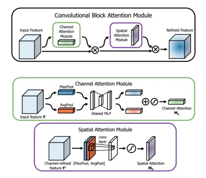
SENet focuses on obtaining attention weights at the channel level, then multiplying them with the original feature map. This article points out that this attention method only considers which layers at the channel level have stronger feedback capabilities, but does not reflect attention in the spatial dimension. CBAM, as a highlight of this article, applies attention simultaneously in both channel and spatial dimensions. Like the SE Module, CBAM can be embedded in most mainstream networks, enhancing the model’s feature extraction ability without significantly increasing computational and parameter loads.

Channel Attention: As shown in the figure above, the input is a feature F of size H×W×C. We first perform global average pooling and max pooling to obtain two channel descriptors of size 1×1×C. These are then sent into a two-layer neural network, where the first layer has C/r neurons with ReLU as the activation function, and the second layer has C neurons. Note that this two-layer neural network is shared. The two features obtained are added together and passed through a Sigmoid activation function to obtain the weight coefficients Mc. Finally, the weight coefficients are multiplied with the original feature F to obtain the new scaled feature. Pseudocode:

def forward(self, x):
    # Use FC to obtain global information, essentially the same as multiplying with Non-local's matrix
    avg_out = self.fc2(self.relu1(self.fc1(self.avg_pool(x))))
    max_out = self.fc2(self.relu1(self.fc1(self.max_pool(x))))
    out = avg_out + max_out
    return self.sigmoid(out)

Spatial Attention: Similar to channel attention, given a feature F’ of size H×W×C, we first perform average pooling and max pooling along the channel dimension to obtain two channel descriptors of size H×W×1, then concatenate these two descriptors along the channel dimension. Afterward, a 7×7 convolution layer with a Sigmoid activation function is applied to obtain the weight coefficients Ms. Finally, the weight coefficients are multiplied with the feature F’ to obtain the new scaled feature. Pseudocode:

def forward(self, x):
    # Use pooling to obtain global information
    avg_out = torch.mean(x, dim=1, keepdim=True)
    max_out, _ = torch.max(x, dim=1, keepdim=True)
    x = torch.cat([avg_out, max_out], dim=1)
    x = self.conv1(x)
    return self.sigmoid(x)

6 DCN v1&v2

Full Name of Plug-in: Deformable Convolutional

From Paper:

v1: [Deformable Convolutional Networks]

https://arxiv.org/pdf/1703.06211.pdf

v2: [Deformable ConvNets v2: More Deformable, Better Results]

https://arxiv.org/pdf/1811.11168.pdf

Core Analysis:

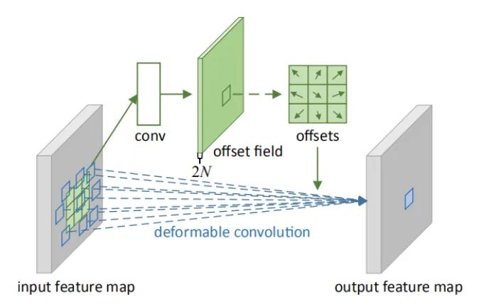
Deformable convolution can be viewed as a combination of deformation and convolution, thus can be used as a plug-in. In many mainstream detection networks, deformable convolution is indeed a feature enhancement tool, and there are many interpretations available online. Compared to traditional fixed-window convolutions, deformable convolution can effectively adapt to geometric shapes since its “local receptive field” is learnable and oriented towards the entire image. This paper also proposes deformable ROI pooling, both methods add extra offsets to the spatial sampling locations without requiring additional supervision, making it a self-supervised process.

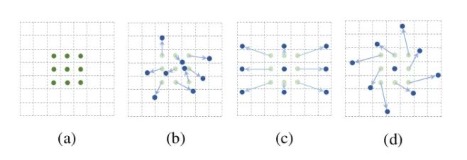
As shown in the figure above, a represents different convolutions, b represents deformable convolution, and the dark points represent the actual sampling locations of the convolution kernel, which are offset from the “standard” positions. c and d represent special forms of deformable convolution, where c is the commonly seen dilated convolution, and d is a convolution with learned rotation characteristics, also enhancing the receptive field.

Deformable convolution is very similar to the STN process; STN learns six parameters for spatial transformation through the network to perform overall transformations on the feature map, aimed at increasing the network’s ability to extract deformations. DCN learns offsets for the entire image, which is a bit more comprehensive than STN. STN is affine transformation, while DCN can perform arbitrary transformations. I won’t include the formulas, as you can directly refer to the code implementation.

Deformable convolution has two versions, V1 and V2, where V2 improves upon V1 by not only learning sampling offsets but also sampling weights. V2 posits that 3X3 sampling points should also have different levels of importance, thus making this processing method more flexible and better at fitting.

Core Code:

def forward(self, x):
    # Learn the offsets, including x and y directions; note that each pixel in each channel has its own x and y offsets
    offset = self.p_conv(x)
    if self.v2: # In V2, an additional weight coefficient is learned, normalized between 0 and 1 using sigmoid
        m = torch.sigmoid(self.m_conv(x))
    # Use offsets to interpolate x, obtaining x_offset
    x_offset = self.interpolate(x,offset)
    if self.v2: # In V2, apply the weight coefficient to the feature map
        m = m.contiguous().permute(0, 2, 3, 1)
        m = m.unsqueeze(dim=1)
        m = torch.cat([m for _ in range(x_offset.size(1))], dim=1)
        x_offset *= m
    out = self.conv(x_offset) # After applying offsets, perform standard convolution
    return out

7 CoordConv

From Paper: An intriguing failing of convolutional neural networks and the CoordConv solution

Paper Link: https://arxiv.org/pdf/1807.03247.pdf

Core Analysis:

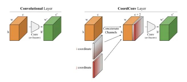
You can see its presence in the Solo semantic segmentation algorithm and Yolov5. This article explores the ability of convolutional networks in coordinate transformations through several small experiments. The issue is that they cannot convert spatial representations into coordinates in Cartesian space. As shown in the figure, we input coordinates (i, j) into a network, requiring it to output a 64×64 image and draw a square or a pixel at those coordinates. However, the network fails to complete this task on the test set, despite it being a task that humans find extremely simple. The analysis reveals that convolution, as a local and weight-sharing filter applied to the input, does not know where each filter is and cannot capture positional information. Therefore, we can assist the convolution by providing it with the position of the filters. We only need to add two channels to the input, one for the i coordinate and another for the j coordinate. The specific approach is shown in the figure above, where two channels are added before passing through the filters. This way, the network gains the ability to perceive spatial location, which is quite remarkable. You can randomly use this module in classification, segmentation, and detection tasks.

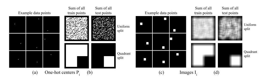
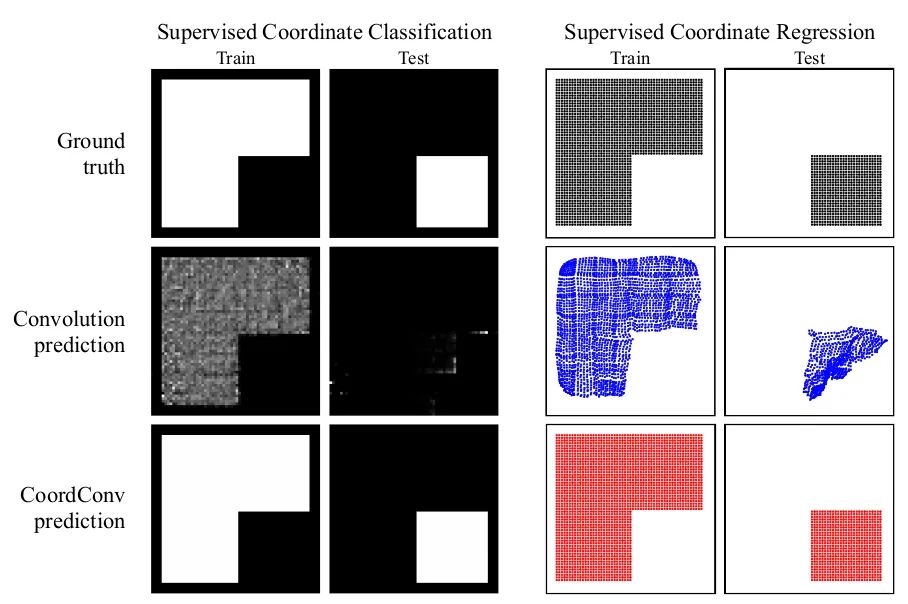
As shown in the first group of images, traditional CNNs struggle with the task of generating images based on coordinate values, performing well on the training set but poorly on the test set. The second group of images demonstrates that after adding CoordConv, the task can be easily completed, showcasing its enhancement of CNN’s spatial perception capabilities.

Core Code:

ins_feat = x # Current instance feature tensor
# Generate linear values from -1 to 1
x_range = torch.linspace(-1, 1, ins_feat.shape[-1], device=ins_feat.device)
y_range = torch.linspace(-1, 1, ins_feat.shape[-2], device=ins_feat.device)
y, x = torch.meshgrid(y_range, x_range) # Generate 2D coordinate grid
y = y.expand([ins_feat.shape[0], 1, -1, -1]) # Expand to the same dimensions as ins_feat
x = x.expand([ins_feat.shape[0], 1, -1, -1])
coord_feat = torch.cat([x, y], 1) # Position features
ins_feat = torch.cat([ins_feat, coord_feat], 1) # Concatenate as input for the next convolution

8 Ghost

Full Name of Plug-in: Ghost module

From Paper: GhostNet: More Features from Cheap Operations

Paper Link: https://arxiv.org/pdf/1911.11907.pdf

Core Analysis:

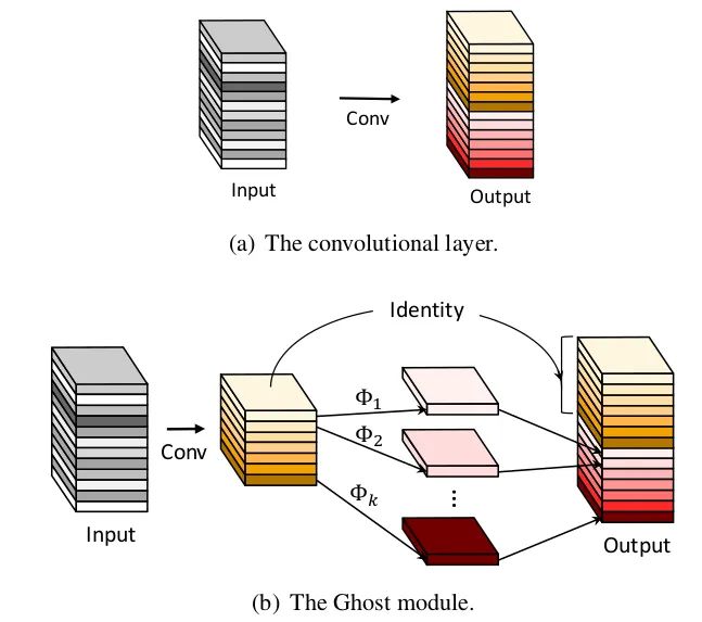
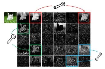
In the ImageNet classification task, GhostNet achieved a Top-1 accuracy of 75.7% with a similar computational load to MobileNetV3’s 75.2%. Its primary innovation is the introduction of the Ghost module. In CNN models, feature maps often contain a lot of redundancy, which is important and necessary. As shown in the figure, the feature maps marked with a “small wrench” contain redundant features. So, can we reduce the number of convolution channels and then generate redundant feature maps through some transformations? This is essentially the idea behind GhostNet.

This article starts from the problem of feature map redundancy, proposing a structure that can generate a large number of feature maps through a small amount of computation (referred to as cheap operations in the paper) – the Ghost Module. The cheap operations are linear transformations, implemented using convolution operations. The specific process is as follows:

• Use fewer convolution operations than originally required; for example, instead of using 64 convolution kernels, use 32, reducing the computational load by half.

• Utilize depthwise separable convolutions to transform the generated feature maps into redundant features.

• Concatenate the features obtained from the above two steps and output them for subsequent processing.

Core Code:

class GhostModule(nn.Module):
    def __init__(self, inp, oup, kernel_size=1, ratio=2, dw_size=3, stride=1, relu=True):
        super(GhostModule, self).__init__()
        self.oup = oup
        init_channels = math.ceil(oup / ratio)
        new_channels = init_channels*(ratio-1)
        self.primary_conv = nn.Sequential(
            nn.Conv2d(inp, init_channels, kernel_size, stride, kernel_size//2, bias=False),
            nn.BatchNorm2d(init_channels),
            nn.ReLU(inplace=True) if relu else nn.Sequential(), )  # Cheap operation, utilizing grouped convolutions for channel separation
        self.cheap_operation = nn.Sequential(
            nn.Conv2d(init_channels, new_channels, dw_size, 1, dw_size//2, groups=init_channels, bias=False),
            nn.BatchNorm2d(new_channels),
            nn.ReLU(inplace=True) if relu else nn.Sequential(),)
    def forward(self, x):
        x1 = self.primary_conv(x)  # Main convolution operation
        x2 = self.cheap_operation(x1) # Cheap transformation operation
        out = torch.cat([x1,x2], dim=1) # Concatenate both outputs
        return out[:,:self.oup,:,:]

9 BlurPool

From Paper: Making Convolutional Networks Shift-Invariant Again

Paper Link: https://arxiv.org/abs/1904.11486

Core Analysis:

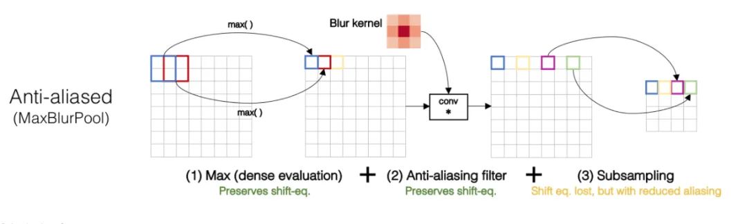
We all know that convolution operations based on sliding windows possess translational invariance, thus it is assumed that CNN networks have translational invariance or equivariance. However, is this truly the case? In practice, CNNs are very sensitive; even a slight change in a pixel or shifting an image by one pixel can lead to significant changes in CNN outputs, even resulting in incorrect predictions. This indicates a lack of robustness. Generally, we use data augmentation to achieve what is termed “invariance”. This article explores the underlying cause of the degradation in invariance, which is primarily due to downsampling; whether through Max Pooling, Average Pooling, or convolutions with stride > 1, any downsampling operation with a stride greater than 1 results in the loss of translational invariance. The figures below illustrate that merely shifting a pixel can lead to a significant difference in the results of Max Pooling.

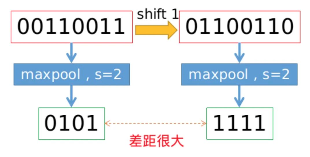
To maintain translational invariance, low-pass filtering can be applied before downsampling. Traditional max pooling can be decomposed into two parts: max pooling with stride = 1 + downsampling. Therefore, the author proposes MaxBlurPool = max + blur + downsampling to replace the original max pooling. Experiments show that while this operation does not completely solve the loss of translational invariance, it significantly alleviates the issue.

Core Code:

class BlurPool(nn.Module):
    def __init__(self, channels, pad_type='reflect', filt_size=4, stride=2, pad_off=0):
        super(BlurPool, self).__init__()
        self.filt_size = filt_size
        self.pad_off = pad_off
        self.pad_sizes = [int(1.*(filt_size-1)/2), int(np.ceil(1.*(filt_size-1)/2)), int(1.*(filt_size-1)/2), int(np.ceil(1.*(filt_size-1)/2))]
        self.pad_sizes = [pad_size+pad_off for pad_size in self.pad_sizes]
        self.stride = stride
        self.off = int((self.stride-1)/2.)
        self.channels = channels    # Define a series of Gaussian kernels
        if(self.filt_size==1):
            a = np.array([1.,])
        elif(self.filt_size==2):
            a = np.array([1., 1.])
        elif(self.filt_size==3):
            a = np.array([1., 2., 1.])
        elif(self.filt_size==4):
            a = np.array([1., 3., 3., 1.])
        elif(self.filt_size==5):
            a = np.array([1., 4., 6., 4., 1.])
        elif(self.filt_size==6):
            a = np.array([1., 5., 10., 10., 5., 1.])
        elif(self.filt_size==7):
            a = np.array([1., 6., 15., 20., 15., 6., 1.])
        filt = torch.Tensor(a[:,None]*a[None,:])
        filt = filt/torch.sum(filt) # Normalization to ensure the amount of information remains constant after blur
        # Store non-grad parameters in buffer
        self.register_buffer('filt', filt[None,None,:,:].repeat((self.channels,1,1,1)))
        self.pad = get_pad_layer(pad_type)(self.pad_sizes)
    def forward(self, inp):
        if(self.filt_size==1):
            if(self.pad_off==0):
                return inp[:,:,::self.stride,::self.stride]
                else:
                return self.pad(inp)[:,:,::self.stride,::self.stride]
        else:
            # Perform blurpool using fixed parameter conv2d+stride
            return F.conv2d(self.pad(inp), self.filt, stride=self.stride, groups=inp.shape[1])

10 RFB

Full Name of Plug-in: Receptive Field Block

From Paper: Receptive Field Block Net for Accurate and Fast Object Detection

Paper Link: https://arxiv.org/abs/1711.07767

Core Analysis:

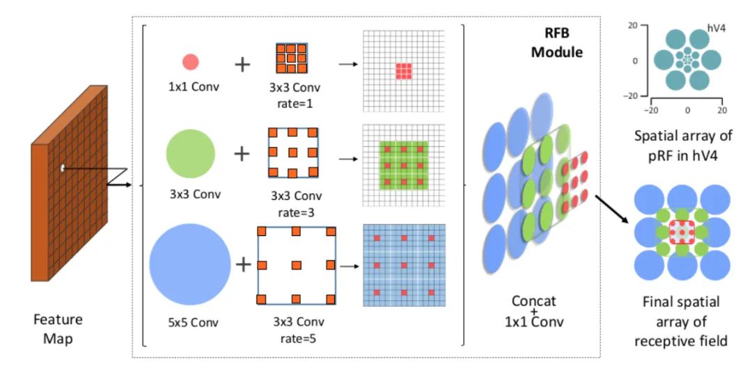
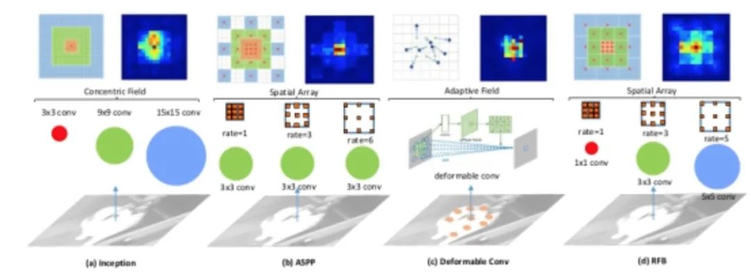
The paper finds that target regions should be close to the center of the receptive field to enhance the model’s robustness to small-scale spatial displacements. Inspired by the RF structure in human vision, this paper proposes the Receptive Field Block (RFB), which enhances the deep feature learning of CNN models, making detection models more accurate. RFB can be viewed as a universal module that can be embedded in most networks. The diagram below illustrates its differences from inception, ASPP, and DCN, which can be seen as a combination of inception and ASPP.

The specific implementation is shown in the diagram below, which is actually similar to ASPP but uses different sizes of convolution kernels as pre-operations for dilated convolutions.

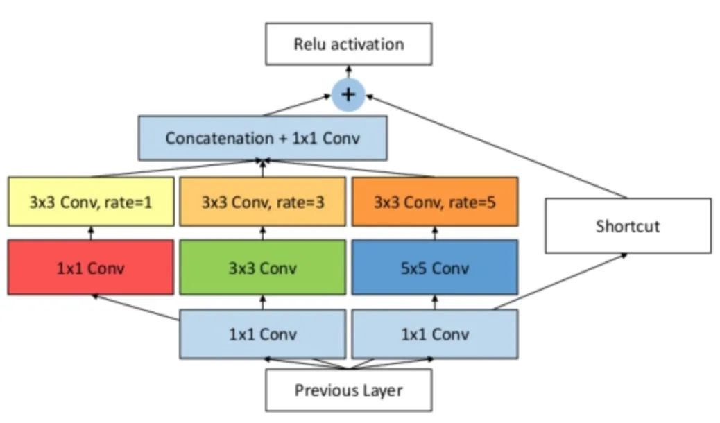
Core Code:

class RFB(nn.Module):
    def __init__(self, in_planes, out_planes, stride=1, scale = 0.1, visual = 1):
        super(RFB, self).__init__()
        self.scale = scale
        self.out_channels = out_planes
        inter_planes = in_planes // 8
        # Branch 0: 1X1 convolution + 3X3 convolution
        self.branch0 = nn.Sequential(conv_bn_relu(in_planes, 2*inter_planes, 1, stride),
                conv_bn_relu(2*inter_planes, 2*inter_planes, 3, 1, visual, visual, False))
        # Branch 1: 1X1 convolution + 3X3 convolution + dilated convolution
        self.branch1 = nn.Sequential(conv_bn_relu(in_planes, inter_planes, 1, 1),
                conv_bn_relu(inter_planes, 2*inter_planes, (3,3), stride, (1,1)),
                conv_bn_relu(2*inter_planes, 2*inter_planes, 3, 1, visual+1,visual+1,False))
        # Branch 2: 1X1 convolution + 3X3 convolution*3 instead of 5X5 convolution + dilated convolution
        self.branch2 = nn.Sequential(conv_bn_relu(in_planes, inter_planes, 1, 1),
                conv_bn_relu(inter_planes, (inter_planes//2)*3, 3, 1, 1),
                conv_bn_relu((inter_planes//2)*3, 2*inter_planes, 3, stride, 1),
                conv_bn_relu(2*inter_planes, 2*inter_planes, 3, 1, 2*visual+1, 2*visual+1,False))
        self.ConvLinear = conv_bn_relu(6*inter_planes, out_planes, 1, 1, False)
        self.shortcut = conv_bn_relu(in_planes, out_planes, 1, stride, relu=False)
        self.relu = nn.ReLU(inplace=False)
    def forward(self,x):
        x0 = self.branch0(x)
        x1 = self.branch1(x)
        x2 = self.branch2(x)
    # Scale fusion
        out = torch.cat((x0,x1,x2),1)
        # 1X1 convolution
        out = self.ConvLinear(out)
        short = self.shortcut(x)
        out = out*self.scale + short
        out = self.relu(out)
        return out

11 ASFF

Full Name of Plug-in: Adaptively Spatial Feature Fusion

From Paper: Adaptively Spatial Feature Fusion Learning Spatial Fusion for Single-Shot Object Detection

Paper Link: https://arxiv.org/abs/1911.09516v1

Core Analysis:

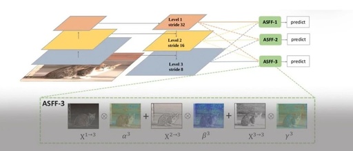
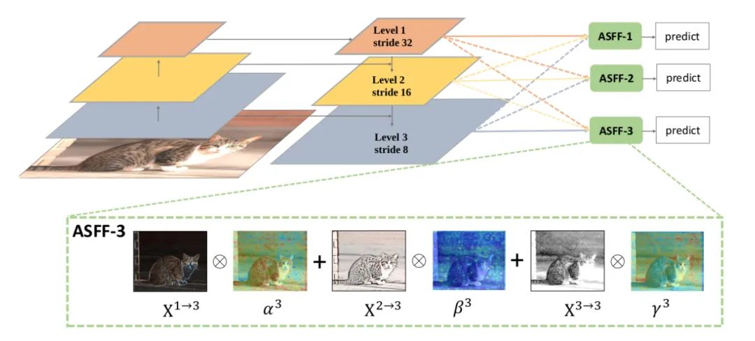
To make better use of high-level semantic features and low-level fine-grained features, many networks adopt FPN to output multi-layer features, but they mostly use concat or element-wise fusion methods. This paper argues that such methods do not fully utilize features of different scales, thus proposing Adaptively Spatial Feature Fusion, an adaptive feature fusion approach. The feature maps output by FPN undergo the following two processes:

Feature Resizing: Feature maps with different scales cannot be fused element-wise, thus resizing is necessary. For upsampling: first, a 1X1 convolution is used for channel compression, followed by interpolation for upsampling the feature map. For downsampling by 1/2: a 3X3 convolution with stride=2 performs both channel compression and feature map reduction. For downsampling by 1/4: a max pooling operation with stride=2 is inserted before a 3X3 convolution with stride=2.

Adaptive Fusion: The feature maps are fused adaptively, as follows:

Where x n→l represents the feature vector at position (i, j) from the n feature map resized to the l scale. Alpha, Beta, and Gamma are spatial attention weights, processed through softmax, as follows:

Code Analysis:

class ASFF(nn.Module):
    def __init__(self, level, rfb=False):
        super(ASFF, self).__init__()
        self.level = level
        # Input channel counts for the three feature layers, modify as needed
        self.dim = [512, 256, 256]
        self.inter_dim = self.dim[self.level]
        # Ensure output channel counts for each layer are consistent
        if level==0:
            self.stride_level_1 = conv_bn_relu(self.dim[1], self.inter_dim, 3, 2)
            self.stride_level_2 = conv_bn_relu(self.dim[2], self.inter_dim, 3, 2)
            self.expand = conv_bn_relu(self.inter_dim, 1024, 3, 1)
        elif level==1:
            self.compress_level_0 = conv_bn_relu(self.dim[0], self.inter_dim, 1, 1)
            self.stride_level_2 = conv_bn_relu(self.dim[2], self.inter_dim, 3, 2)
            self.expand = conv_bn_relu(self.inter_dim, 512, 3, 1)
        elif level==2:
            self.compress_level_0 = conv_bn_relu(self.dim[0], self.inter_dim, 1, 1)
            if self.dim[1] != self.dim[2]:
                self.compress_level_1 = conv_bn_relu(self.dim[1], self.inter_dim, 1, 1)
            self.expand = add_conv(self.inter_dim, 256, 3, 1)
        compress_c = 8 if rfb else 16          self.weight_level_0 = conv_bn_relu(self.inter_dim, compress_c, 1, 1)
        self.weight_level_1 = conv_bn_relu(self.inter_dim, compress_c, 1, 1)
        self.weight_level_2 = conv_bn_relu(self.inter_dim, compress_c, 1, 1)
        self.weight_levels = nn.Conv2d(compress_c*3, 3, 1, 1, 0)
  # Scale sizes level_0 < level_1 < level_2    def forward(self, x_level_0, x_level_1, x_level_2):
        # Feature Resizing process
        if self.level==0:
            level_0_resized = x_level_0
            level_1_resized = self.stride_level_1(x_level_1)
            level_2_downsampled_inter =F.max_pool2d(x_level_2, 3, stride=2, padding=1)
            level_2_resized = self.stride_level_2(level_2_downsampled_inter)
        elif self.level==1:
            level_0_compressed = self.compress_level_0(x_level_0)
            level_0_resized =F.interpolate(level_0_compressed, 2, mode='nearest')
            level_1_resized =x_level_1
            level_2_resized =self.stride_level_2(x_level_2)
        elif self.level==2:
            level_0_compressed = self.compress_level_0(x_level_0)
            level_0_resized =F.interpolate(level_0_compressed, 4, mode='nearest')
            if self.dim[1] != self.dim[2]:
                level_1_compressed = self.compress_level_1(x_level_1)
                level_1_resized = F.interpolate(level_1_compressed, 2, mode='nearest')
            else:
                level_1_resized =F.interpolate(x_level_1, 2, mode='nearest')
            level_2_resized =x_level_2
    # Fusion weights are also learned from the network
        level_0_weight_v = self.weight_level_0(level_0_resized)
        level_1_weight_v = self.weight_level_1(level_1_resized)
        level_2_weight_v = self.weight_level_2(level_2_resized)
        levels_weight_v = torch.cat((level_0_weight_v, level_1_weight_v,                                     level_2_weight_v),1)
        levels_weight = self.weight_levels(levels_weight_v)
        levels_weight = F.softmax(levels_weight, dim=1)   # Alpha generated
    # Adaptive fusion
        fused_out_reduced = level_0_resized * levels_weight[:,0:1,:,:]+
                            level_1_resized * levels_weight[:,1:2,:,:]+
                            level_2_resized * levels_weight[:,2:,:,:]
        out = self.expand(fused_out_reduced)
        return out

Conclusion

This article reviews some cleverly designed and practical CNN plug-ins in recent years, hoping that everyone can apply them in their actual projects.