Introduction “Plugins” are enhancements that can be easily integrated into existing systems, truly embodying the plug-and-play concept. The “plugins” discussed in this article can enhance the CNN’s ability to handle transformations like translation, rotation, and scale, as well as multi-scale feature extraction, and can be found in many SOTA networks.

Pytorch training camp, master coding implementation in two weeks

Comprehensive tutorials on various CV directions and deployment frameworks

CV full-stack guidance class, basic introductory class, and thesis guidance class are fully online!!

Overview

This article reviews some practical and elegantly designed “plugins” for CNN networks. A “plugin” should not change the main structure of the network but can be easily embedded into mainstream networks to enhance the network’s feature extraction capabilities, achieving plug-and-play functionality. There are many similar assessments in networks that claim to offer plug-and-play capabilities without hassle. However, based on my experience and research, I found that many plugins are impractical, non-generalizable, or even ineffective, hence this article.

First, my understanding is: since it is a “plugin”, it should be an enhancement that is easy to embed and implement, truly plug-and-play. The “plugins” discussed in this article can be seen in many SOTA networks. They are commendable “plugins” that can genuinely achieve plug-and-play functionality. In short, they are “plugins” that work. Many “plugins” have been introduced to enhance CNN capabilities, such as transformation capabilities like translation, rotation, scaling, multi-scale feature extraction, receptive field capabilities, and spatial position perception capabilities.

Shortlisted Plugins: STN, ASPP, Non-local, SE, CBAM, DCNv1&v2, CoordConv, Ghost, BlurPool, RFB, ASFF

1. STN

Originating Paper: Spatial Transformer Networks

Paper Link: https://arxiv.org/pdf/1506.02025.pdf

Core Analysis:

In tasks like OCR, you will often see its presence. For CNN networks, we hope they possess a certain invariance to the object’s pose and position. This means they can adapt to certain pose and position changes on the test set. Invariance can effectively improve the model’s generalization ability. Although CNNs use sliding-window convolution operations that provide some degree of translational invariance, many studies have found that downsampling can destroy this invariance. Thus, the network’s invariance capability is considered weak, let alone invariance to rotation, scale, and illumination. Generally, we use data augmentation to achieve network “invariance”.

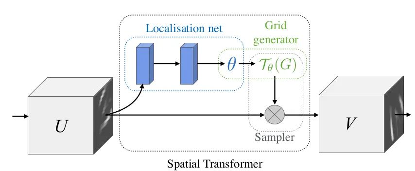
This article proposes the STN module, which explicitly embeds spatial transformations into the network to enhance the network’s invariance to rotation, translation, and scale. It can be understood as an “alignment” operation. The structure of STN is shown in the figure above, where each STN module consists of a Localisation net, Grid generator, and Sampler. The Localisation net learns the parameters for spatial transformation, which are the six parameters in the equation. The Grid generator is responsible for coordinate mapping. The Sampler collects pixels using bilinear interpolation.

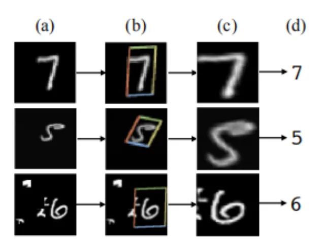
The significance of STN is that it can correct the original image into the ideal image desired by the network, and this process occurs in an unsupervised manner, meaning the transformation parameters are learned spontaneously without requiring labeled information. This module is an independent module that can be inserted at any position in the CNN. It meets the requirements for this “plugin” review.

Core Code:

class SpatialTransformer(nn.Module):    def __init__(self, spatial_dims):        super(SpatialTransformer, self).__init__()        self._h, self._w = spatial_dims         self.fc1 = nn.Linear(32*4*4, 1024) # Set according to your network parameters        self.fc2 = nn.Linear(1024, 6)    def forward(self, x):         batch_images = x # Save a copy of the original data        x = x.view(-1, 32*4*4)        # Use FC structure to learn the 6 parameters        x = self.fc1(x)        x = self.fc2(x)         x = x.view(-1, 2,3) # 2x3        # Generate sampling points using affine_grid        affine_grid_points = F.affine_grid(x, torch.Size((x.size(0), self._in_ch, self._h, self._w)))        # Apply sampling points to the original data        rois = F.grid_sample(batch_images, affine_grid_points)        return rois, affine_grid_points

2. ASPP

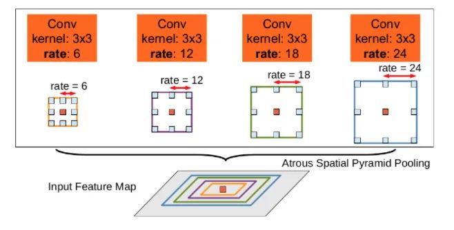
Full Name of Plugin: Atrous Spatial Pyramid Pooling

Originating Paper: DeepLab: Semantic Image Segmentation with Deep Convolutional Nets, Atrous Conv

Paper Link: https://arxiv.org/pdf/1606.00915.pdf

Core Analysis:

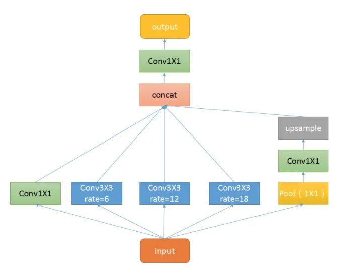
This plugin is a spatial pyramid pooling module with atrous convolution, mainly proposed to enhance the network’s receptive field and introduce multi-scale information. We know that semantic segmentation networks often deal with high-resolution images, which requires our networks to have a sufficient receptive field to cover the target object. Basic CNN networks achieve receptive fields by stacking convolutional layers and performing upsampling operations. This module can control the receptive field without changing the feature map size, which is beneficial for extracting multi-scale information. The rate controls the size of the receptive field; the larger the rate, the larger the receptive field.

ASPP mainly consists of the following parts: 1. A global average pooling layer to obtain image-level features, followed by a 1×1 convolution, and then bilinearly interpolated to the original size; 2. A 1×1 convolution layer, and three 3×3 atrous convolutions; 3. The features from five different scales are concatenated along the channel dimension and then passed through a 1×1 convolution for fusion output.

Core Code:

class ASPP(nn.Module):    def __init__(self, in_channel=512, depth=256):        super(ASPP,self).__init__()        self.mean = nn.AdaptiveAvgPool2d((1, 1))        self.conv = nn.Conv2d(in_channel, depth, 1, 1)        self.atrous_block1 = nn.Conv2d(in_channel, depth, 1, 1)        # Convolutions with different dilation rates        self.atrous_block6 = nn.Conv2d(in_channel, depth, 3, 1, padding=6, dilation=6)        self.atrous_block12 = nn.Conv2d(in_channel, depth, 3, 1, padding=12, dilation=12)        self.atrous_block18 = nn.Conv2d(in_channel, depth, 3, 1, padding=18, dilation=18)        self.conv_1x1_output = nn.Conv2d(depth * 5, depth, 1, 1)    def forward(self, x):        size = x.shape[2:]     # Pooling branch        image_features = self.mean(x)        image_features = self.conv(image_features)        image_features = F.upsample(image_features, size=size, mode='bilinear')     # Convolutions with different dilation rates        atrous_block1 = self.atrous_block1(x)        atrous_block6 = self.atrous_block6(x)        atrous_block12 = self.atrous_block12(x)        atrous_block18 = self.atrous_block18(x)        # Merge features from all scales     x = torch.cat([image_features, atrous_block1, atrous_block6,atrous_block12, atrous_block18], dim=1)        # Use 1x1 convolution to fuse features for output        x = self.conv_1x1_output(x)        return net

3. Non-local

Originating Paper: Non-local Neural Networks

Paper Link: https://arxiv.org/abs/1711.07971

Core Analysis:

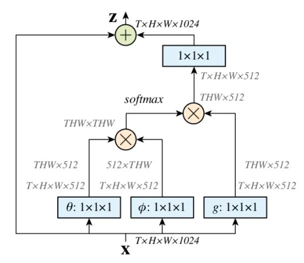
Non-Local is an attention mechanism and an easy-to-integrate module. Local primarily refers to the receptive field; for instance, in the convolution and pooling operations in CNNs, the receptive field size is determined by the filter size, and we often use 3×3 convolution layers stacked, which only consider local areas, hence local operations. In contrast, non-local operations can have a much larger receptive field, potentially encompassing a global area instead of just a local region. Capturing long-range dependencies, i.e., establishing connections between pixels that are a certain distance apart in an image, is a form of attention mechanism. The so-called attention mechanism generates a saliency map, where attention corresponds to salient regions that the network needs to focus on.

• First, perform a 1×1 convolution on the input feature map to compress the channel number, obtaining features.
• Then reshape the dimensions of the three features and perform matrix multiplication to obtain a covariance-like matrix, which is to calculate the self-correlation of the features, i.e., establish the relationships between each pixel in a frame and all other pixels in all frames.
• Next, apply a softmax operation on the self-correlation features to obtain weights ranging from 0 to 1, which are the self-attention coefficients we need.
• Finally, multiply the attention coefficients back onto the feature matrix g and add this to the original input feature map X as a residual output.

Here, let’s understand with a simple example, assuming g is (we will temporarily ignore the batch and channel dimensions):

g = torch.tensor([[1, 2],                           [3, 4]).view(-1, 1).float()

And:

theta = torch.tensor([2, 4, 6, 8]).view(-1, 1)

And:

phi = torch.tensor([7, 5, 3, 1]).view(1, -1)

Then, the matrix multiplication is as follows:

tensor([[14., 10.,  6.,  2.],                [28., 20., 12.,  4.],                [42., 30., 18.,  6.],                [56., 40., 24.,  8.]])

After softmax(dim=-1), it results in the following, where each row represents the importance of elements in g, with larger values in the front indicating that the network should pay more attention to those elements:

tensor([[9.8168e-01, 1.7980e-02, 3.2932e-04, 6.0317e-06],                [9.9966e-01, 3.3535e-04, 1.1250e-07, 3.7739e-11],                [9.9999e-01, 6.1442e-06, 3.7751e-11, 2.3195e-16],                [1.0000e+00, 1.1254e-07, 1.2664e-14, 1.4252e-21]])

After applying attention, the overall values converge towards 1:

tensor([[1.0187, 1.0003],                [1.0000, 1.0000]])

Core Code:

class NonLocal(nn.Module):    def __init__(self, channel):        super(NonLocalBlock, self).__init__()        self.inter_channel = channel // 2        self.conv_phi = nn.Conv2d(channel, self.inter_channel, 1, 1,0, False)        self.conv_theta = nn.Conv2d(channel, self.inter_channel, 1, 1,0, False)        self.conv_g = nn.Conv2d(channel, self.inter_channel, 1, 1, 0, False)        self.softmax = nn.Softmax(dim=1)        self.conv_mask = nn.Conv2d(self.inter_channel, channel, 1, 1, 0, False)    def forward(self, x):        # [N, C, H , W]        b, c, h, w = x.size()        # Get phi features, dimension [N, C/2, H * W], retaining batch and channel dimensions        x_phi = self.conv_phi(x).view(b, c, -1)        # Get theta features, dimension [N, H * W, C/2]        x_theta = self.conv_theta(x).view(b, c, -1).permute(0, 2, 1).contiguous()        # Get g features, dimension [N, H * W, C/2]        x_g = self.conv_g(x).view(b, c, -1).permute(0, 2, 1).contiguous()        # Matrix multiplication of phi and theta, [N, H * W, H * W]        mul_theta_phi = torch.matmul(x_theta, x_phi)        # Softmax to scale between 0 and 1        mul_theta_phi = self.softmax(mul_theta_phi)        # Matrix multiplication with g features, [N, H * W, C/2]        mul_theta_phi_g = torch.matmul(mul_theta_phi, x_g)        # [N, C/2, H, W]        mul_theta_phi_g = mul_theta_phi_g.permute(0, 2, 1).contiguous().view(b, self.inter_channel, h, w)        # 1x1 convolution to expand channel numbers        mask = self.conv_mask(mul_theta_phi_g)        out = mask + x # Residual connection        return out

4. SE

Originating Paper: Squeeze-and-Excitation Networks

Paper Link: https://arxiv.org/pdf/1709.01507.pdf

Core Analysis:

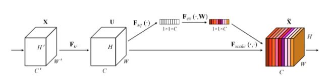
This paper is the champion entry of the last ImageNet competition, and you will see its presence in many classic network architectures, such as Mobilenet v3. It is essentially a channel attention mechanism. Due to feature compression and the presence of FC, the captured channel attention features contain global information. This paper proposes a new structural unit—the “Squeeze-and-Excitation (SE)” module, which can adaptively adjust the feature response values of each channel and model the internal dependencies between channels. The steps are as follows:

• Squeeze: Compress features along the spatial dimension, transforming each 2D feature channel into a single value, which has a global receptive field.

• Excitation: Each feature channel generates a weight representing the importance of that feature channel.

• Reweight: The weights output from Excitation are treated as the importance of each feature channel and are applied to each channel via multiplication.

Core Code:

class SE_Block(nn.Module):    def __init__(self, ch_in, reduction=16):        super(SE_Block, self).__init__()        self.avg_pool = nn.AdaptiveAvgPool2d(1)  # Global adaptive pooling        self.fc = nn.Sequential(            nn.Linear(ch_in, ch_in // reduction, bias=False),            nn.ReLU(inplace=True),            nn.Linear(ch_in // reduction, ch_in, bias=False),            nn.Sigmoid()        )    def forward(self, x):        b, c, _, _ = x.size()        y = self.avg_pool(x).view(b, c) # Squeeze operation        y = self.fc(y).view(b, c, 1, 1) # FC to obtain channel attention weights, containing global information        return x * y.expand_as(x) # Attention applied to each channel

5. CBAM

Originating Paper: CBAM: Convolutional Block Attention Module

Paper Link: https://openaccess.thecvf.com/content_ECCV_2018/papers/Sanghyun_Woo_Convolutional_Block_Attention_ECCV_2018_paper.pdf

Core Analysis:

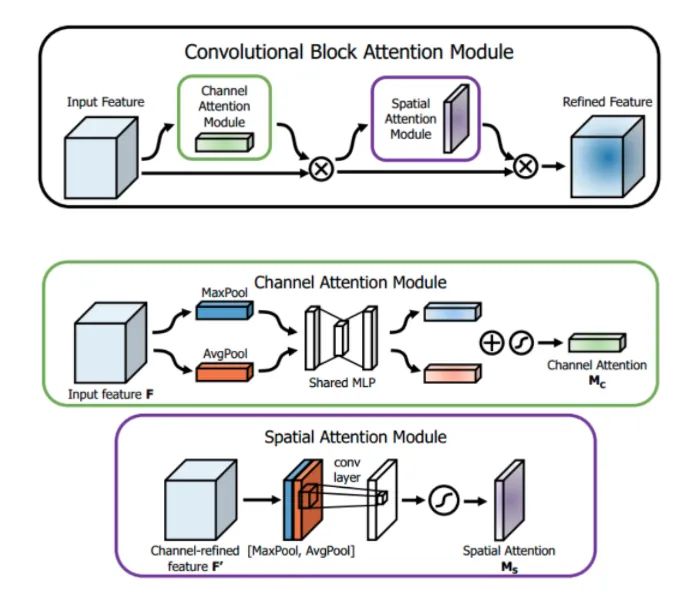
While SENet focuses on obtaining attention weights on the channel dimension of the feature map and then multiplying these with the original feature map, this article points out that this attention method only considers which layers have stronger feedback capabilities at the channel level, but does not reflect attention in the spatial dimension. CBAM, as the highlight of this article, applies attention simultaneously in both channel and spatial dimensions. Like the SE Module, CBAM can be embedded into most mainstream networks without significantly increasing computational or parameter loads, thereby enhancing the model’s feature extraction capabilities.

Channel Attention: As shown in the figure above, the input is a feature F of size H×W×C. We first apply global average pooling and max pooling to obtain two 1×1×C channel descriptors. These are then fed into a two-layer neural network, with the first layer having C/r neurons and the activation function being Relu, and the second layer having C neurons. Note that this two-layer neural network is shared. The two resulting features are summed and passed through a Sigmoid activation function to obtain the weight coefficient Mc. Finally, the weight coefficient is multiplied by the original feature F to obtain the scaled new feature. Pseudocode:

def forward(self, x):    # Use FC to obtain global information, essentially similar to the matrix multiplication in Non-local    avg_out = self.fc2(self.relu1(self.fc1(self.avg_pool(x))))    max_out = self.fc2(self.relu1(self.fc1(self.max_pool(x))))    out = avg_out + max_out    return self.sigmoid(out)

Spatial Attention: Similar to channel attention, given a feature F’ of size H×W×C, we first perform average pooling and max pooling along the channel dimension to obtain two H×W×1 channel descriptors. We then concatenate these two descriptors along the channel dimension. After that, we pass the concatenated descriptor through a 7×7 convolution layer with a Sigmoid activation function to obtain the weight coefficient Ms. Finally, we multiply the weight coefficient with the feature F’ to obtain the scaled new feature. Pseudocode:

def forward(self, x):    # Here, we use pooling to obtain global information    avg_out = torch.mean(x, dim=1, keepdim=True)    max_out, _ = torch.max(x, dim=1, keepdim=True)    x = torch.cat([avg_out, max_out], dim=1)    x = self.conv1(x)    return self.sigmoid(x)

6. DCN v1&v2

Full Name of Plugin: Deformable Convolutional

Originating Paper:

v1: [Deformable Convolutional Networks]

https://arxiv.org/pdf/1703.06211.pdf

v2: [Deformable ConvNets v2: More Deformable, Better Results]

https://arxiv.org/pdf/1811.11168.pdf

Core Analysis:

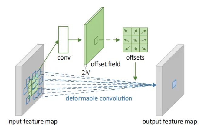
Deformable convolution can be seen as a combination of deformation and convolution, thus can be used as a plugin. In many mainstream detection networks, deformable convolution is indeed a magic tool for increasing performance, and there are numerous interpretations available online. Compared to traditional fixed-window convolutions, deformable convolution can effectively adapt to geometric shapes because its “local receptive field” is learnable and oriented towards the entire image. This paper also proposes deformable ROI pooling, both methods add additional offsets to the spatial sampling locations without requiring extra supervision, making it a self-supervised process.

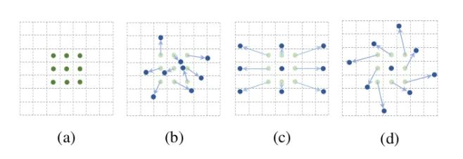
As shown in the figure above, a represents different convolutions, b represents deformable convolution, where the dark points indicate the actual sampling positions of the convolution kernel, which are offset from the “standard” positions. c and d represent special forms of deformable convolution, where c is the common dilated convolution, and d is the convolution with learning rotation characteristics, which also enhances the receptive field capability.

Deformable convolution and STN processes are very similar; STN uses the network to learn the six parameters of spatial transformation to perform overall transformations on the feature map, aiming to enhance the network’s ability to extract deformations. DCN uses the network to learn offsets for the entire image, which is slightly more “comprehensive” than STN. STN is affine transformation, while DCN allows for arbitrary transformations. The formulas are not included here; please refer directly to the code implementation process.

Deformable convolution has two versions: V1 and V2, where V2 improves upon V1 by not only learning sampling offsets but also learning sampling weights. V2 posits that the 3×3 sampling points should also have different levels of importance, making this processing method more flexible and fitting.

Core Code:

def forward(self, x):    # Learn offsets, including x and y directions, note that each pixel in each channel has an x and y offset    offset = self.p_conv(x)    if self.v2: # In V2, an additional weight coefficient is learned and scaled to between 0 and 1 using sigmoid        m = torch.sigmoid(self.m_conv(x))    # Use offsets to interpolate x, obtaining the offset x_offset    x_offset = self.interpolate(x,offset)    if self.v2: # In V2, the weight coefficient is applied to the feature map        m = m.contiguous().permute(0, 2, 3, 1)        m = m.unsqueeze(dim=1)        m = torch.cat([m for _ in range(x_offset.size(1))], dim=1)        x_offset *= m    out = self.conv(x_offset) # Standard convolution process after applying the offset    return out

7. CoordConv

Originating Paper: An intriguing failing of convolutional neural networks and the CoordConv solution

Paper Link: https://arxiv.org/pdf/1807.03247.pdf

Core Analysis:

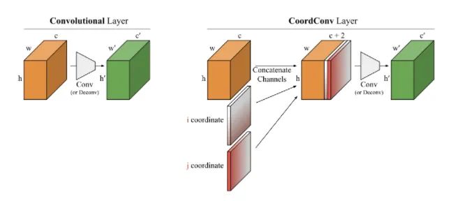
You can see its presence in the Solo semantic segmentation algorithm and Yolov5. This article explores the ability of convolutional networks to perform coordinate transformations based on several small experiments. It highlights their inability to convert spatial representations into coordinates in Cartesian space. As shown in the figure below, we input (i, j) coordinates into a network, requiring it to output a 64×64 image and draw a square or a pixel at the coordinate, yet the network fails to accomplish this on the test set, despite this being a task that is trivial for humans. The reason for this failure is that convolution, being a local, weight-sharing filter applied to inputs, does not know the position of each filter and cannot capture location information. Thus, we can assist the convolution by providing it with positional information about the filters. We simply need to add two channels to the input: one for the i coordinate and one for the j coordinate. The specific method is illustrated in the figure above, where two channels are added before inputting into the filter. This enables the network to possess spatial position information—quite remarkable! You can use this plugin randomly in classification, segmentation, detection, and other tasks.

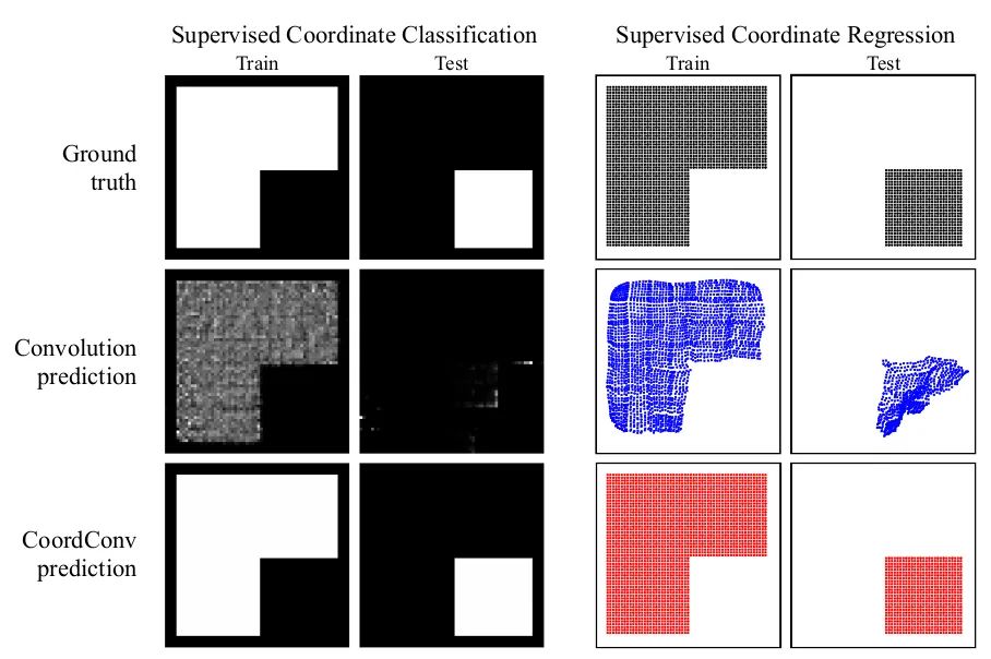
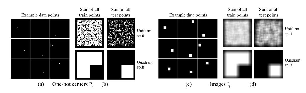
In the first set of images above, the traditional CNN struggles to generate images based on coordinate values during training, resulting in poor performance on the test set. After adding CoordConv in the second set of images, the task can be easily accomplished, demonstrating its enhancement of the CNN’s spatial perception capabilities.

Core Code:

ins_feat = x # Current instance feature tensor# Generate linear values from -1 to 1x_range = torch.linspace(-1, 1, ins_feat.shape[-1], device=ins_feat.device)y_range = torch.linspace(-1, 1, ins_feat.shape[-2], device=ins_feat.device)y, x = torch.meshgrid(y_range, x_range) # Generate 2D coordinate gridy = y.expand([ins_feat.shape[0], 1, -1, -1]) # Expand to match ins_feat dimensionsx = x.expand([ins_feat.shape[0], 1, -1, -1])coord_feat = torch.cat([x, y], 1) # Position featuresins_feat = torch.cat([ins_feat, coord_feat], 1) # Concatenate as input for the next convolution

8. Ghost

Full Name of Plugin: Ghost Module

Originating Paper: GhostNet: More Features from Cheap Operations

Paper Link: https://arxiv.org/pdf/1911.11907.pdf

Core Analysis:

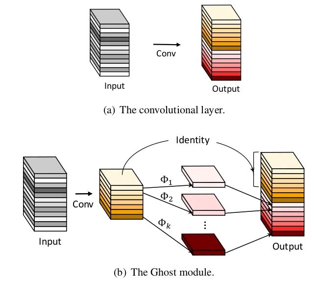
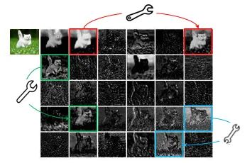
In the ImageNet classification task, GhostNet achieved a Top-1 accuracy of 75.7%, surpassing MobileNetV3’s 75.2% under similar computational loads. Its main innovation is the introduction of the Ghost module. In CNN models, feature maps often contain a lot of redundancy, which is indeed important and necessary. As illustrated in the diagram, the feature maps marked with “small wrenches” exhibit redundant features. So, can we reduce the number of convolution channels and then generate redundant feature maps through some transformation? This is precisely the idea behind GhostNet.

This article addresses the redundancy issue in feature maps by proposing a structure that can generate a large number of feature maps through minimal computation (referred to as cheap operations in the paper)—the Ghost Module. The cheap operations involve linear transformations, with convolution operations implemented in the paper. The specific process is as follows:

• Use fewer convolution operations than originally needed; for instance, instead of using 64 convolution kernels, only 32 are used, halving the computational load.

• Utilize depthwise separable convolutions to transform redundant features from the above step.

• Concatenate the features obtained from the above two steps for output, feeding them into subsequent layers.

Core Code:

class GhostModule(nn.Module):    def __init__(self, inp, oup, kernel_size=1, ratio=2, dw_size=3, stride=1, relu=True):        super(GhostModule, self).__init__()        self.oup = oup        init_channels = math.ceil(oup / ratio)        new_channels = init_channels*(ratio-1)        self.primary_conv = nn.Sequential(            nn.Conv2d(inp, init_channels, kernel_size, stride, kernel_size//2, bias=False),            nn.BatchNorm2d(init_channels),            nn.ReLU(inplace=True) if relu else nn.Sequential(), )  # Cheap operation, utilizing grouped convolutions for channel separation        self.cheap_operation = nn.Sequential(            nn.Conv2d(init_channels, new_channels, dw_size, 1, dw_size//2, groups=init_channels, bias=False),            nn.BatchNorm2d(new_channels),            nn.ReLU(inplace=True) if relu else nn.Sequential(),)    def forward(self, x):        x1 = self.primary_conv(x)  # Main convolution operation        x2 = self.cheap_operation(x1) # Cheap transformation operation        out = torch.cat([x1,x2], dim=1) # Concatenate both outputs        return out[:,:self.oup,:,:]

9. BlurPool

Originating Paper: Making Convolutional Networks Shift-Invariant Again

Paper Link: https://arxiv.org/abs/1904.11486

Core Analysis:

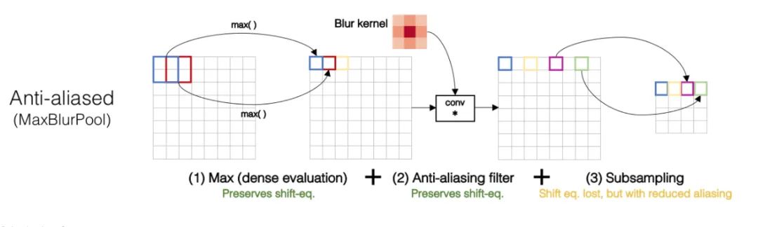
We all know that convolution operations based on sliding windows are translationally invariant, and thus CNN networks are assumed to possess translational invariance or equivariance. However, is this really the case? In practice, CNNs are highly sensitive; a slight change to an input image, even moving it by one pixel, can cause significant changes in the CNN’s output, even leading to incorrect predictions. This indicates a lack of robustness. Typically, we achieve so-called invariance through data augmentation. This paper finds that the degradation of invariance is fundamentally due to downsampling—whether it is Max Pooling, Average Pooling, or convolutions with stride > 1, any downsampling operation involving a stride greater than 1 leads to a loss of translational invariance. The following figure illustrates how even moving a pixel can result in significant differences in the output of Max Pooling.

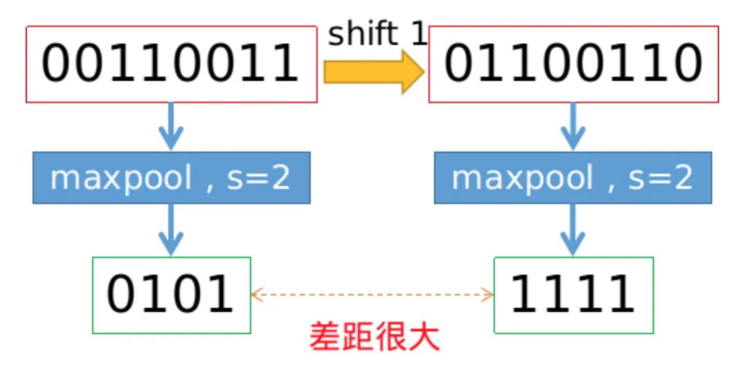
To maintain translational invariance, low-pass filtering can be performed before downsampling. Traditional max pooling can be decomposed into two parts: max with stride = 1 + downsampling. Therefore, the authors propose MaxBlurPool = max + blur + downsampling to replace the original max pooling. Experiments show that while this operation does not completely solve the loss of translational invariance, it significantly alleviates the issue.

Core Code:

class BlurPool(nn.Module):    def __init__(self, channels, pad_type='reflect', filt_size=4, stride=2, pad_off=0):        super(BlurPool, self).__init__()        self.filt_size = filt_size        self.pad_off = pad_off        self.pad_sizes = [int(1.*(filt_size-1)/2), int(np.ceil(1.*(filt_size-1)/2)), int(1.*(filt_size-1)/2), int(np.ceil(1.*(filt_size-1)/2))]        self.pad_sizes = [pad_size+pad_off for pad_size in self.pad_sizes]        self.stride = stride        self.off = int((self.stride-1)/2.)        self.channels = channels    # Define a series of Gaussian kernels        if(self.filt_size==1):            a = np.array([1.,])        elif(self.filt_size==2):            a = np.array([1., 1.])        elif(self.filt_size==3):            a = np.array([1., 2., 1.])        elif(self.filt_size==4):                a = np.array([1., 3., 3., 1.])        elif(self.filt_size==5):                a = np.array([1., 4., 6., 4., 1.])        elif(self.filt_size==6):                a = np.array([1., 5., 10., 10., 5., 1.])        elif(self.filt_size==7):                a = np.array([1., 6., 15., 20., 15., 6., 1.])        filt = torch.Tensor(a[:,None]*a[None,:])        filt = filt/torch.sum(filt) # Normalization to ensure the amount of information remains unchanged after blur        # Store non-grad parameters using buffer        self.register_buffer('filt', filt[None,None,:,:].repeat((self.channels,1,1,1)))        self.pad = get_pad_layer(pad_type)(self.pad_sizes)    def forward(self, inp):        if(self.filt_size==1):            if(self.pad_off==0):                return inp[:,:,::self.stride,::self.stride]                else:                return self.pad(inp)[:,:,::self.stride,::self.stride]        else:            # Implement blur pooling using fixed-parameter conv2d+stride            return F.conv2d(self.pad(inp), self.filt, stride=self.stride, groups=inp.shape[1])

10. RFB

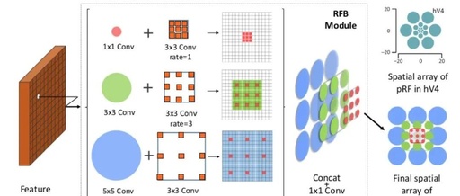
Full Name of Plugin: Receptive Field Block

Originating Paper: Receptive Field Block Net for Accurate and Fast Object Detection

Paper Link: https://arxiv.org/abs/1711.07767

Core Analysis:

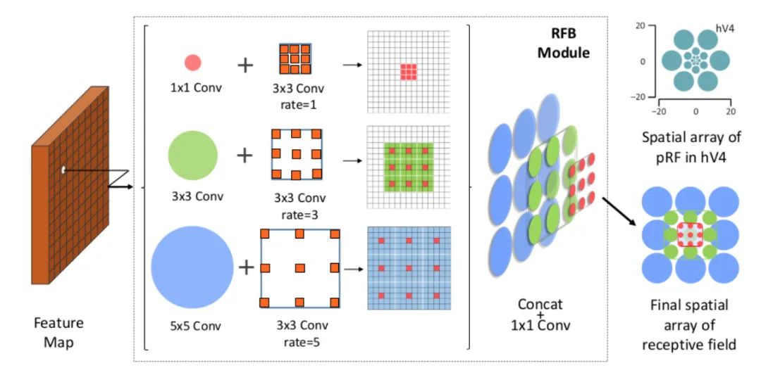
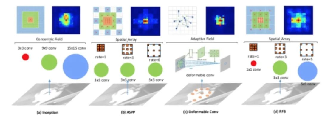
The paper finds that the target region should be as close to the center of the receptive field as possible, which helps enhance the model’s robustness to small-scale spatial displacements. Inspired by the RF structure of human vision, this paper proposes the Receptive Field Block (RFB), which strengthens the capability of deep features learned by CNN models, making detection models more accurate. RFB can be used as a general module embedded in most networks. The following figure illustrates its differences from inception, ASPP, and DCN, showing that it can be viewed as a combination of inception and ASPP.

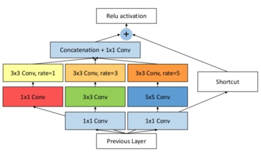
The specific implementation is shown in the figure below, which is similar to ASPP but uses different sized convolution kernels as a precursor to dilated convolutions.

Core Code:

class RFB(nn.Module):    def __init__(self, in_planes, out_planes, stride=1, scale = 0.1, visual = 1):        super(RFB, self).__init__()        self.scale = scale        self.out_channels = out_planes        inter_planes = in_planes // 8        # Branch 0: 1x1 convolution + 3x3 convolution        self.branch0 = nn.Sequential(conv_bn_relu(in_planes, 2*inter_planes, 1, stride),                conv_bn_relu(2*inter_planes, 2*inter_planes, 3, 1, visual, visual, False))        # Branch 1: 1x1 convolution + 3x3 convolution + dilated convolution        self.branch1 = nn.Sequential(conv_bn_relu(in_planes, inter_planes, 1, 1),                conv_bn_relu(inter_planes, 2*inter_planes, (3,3), stride, (1,1)),                conv_bn_relu(2*inter_planes, 2*inter_planes, 3, 1, visual+1,visual+1,False))        # Branch 2: 1x1 convolution + 3x3 convolution*3 instead of 5x5 convolution + dilated convolution        self.branch2 = nn.Sequential(conv_bn_relu(in_planes, inter_planes, 1, 1),                conv_bn_relu(inter_planes, (inter_planes//2)*3, 3, 1, 1),                conv_bn_relu((inter_planes//2)*3, 2*inter_planes, 3, stride, 1),                conv_bn_relu(2*inter_planes, 2*inter_planes, 3, 1, 2*visual+1, 2*visual+1,False))        self.ConvLinear = conv_bn_relu(6*inter_planes, out_planes, 1, 1, False)        self.shortcut = conv_bn_relu(in_planes, out_planes, 1, stride, relu=False)        self.relu = nn.ReLU(inplace=False)    def forward(self,x):        x0 = self.branch0(x)        x1 = self.branch1(x)        x2 = self.branch2(x)    # Scale fusion        out = torch.cat((x0,x1,x2),1)        # 1x1 convolution        out = self.ConvLinear(out)        short = self.shortcut(x)        out = out*self.scale + short        out = self.relu(out)        return out

11. ASFF

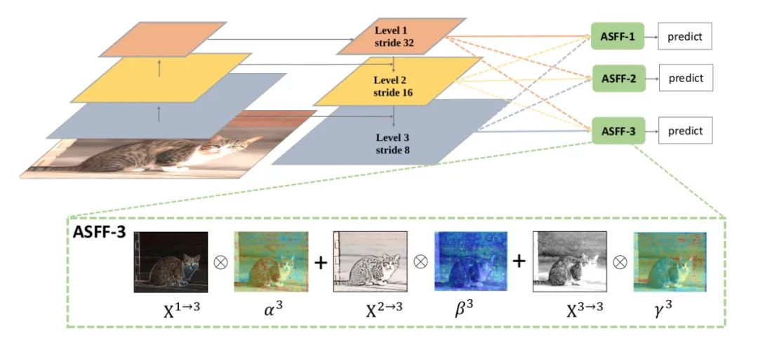
Full Name of Plugin: Adaptively Spatial Feature Fusion

Originating Paper: Adaptively Spatial Feature Fusion Learning Spatial Fusion for Single-Shot Object Detection

Paper Link: https://arxiv.org/abs/1911.09516v1

Core Analysis:

To fully utilize high-level semantic features and low-level fine-grained features, many networks adopt a feature pyramid network (FPN) approach to output multi-layer features. However, they often use concatenation or element-wise fusion methods, which this paper argues do not adequately leverage features of different scales. Thus, it proposes Adaptively Spatial Feature Fusion, a self-adaptive feature fusion method. The feature maps output by FPN undergo the following two processes:

Feature Resizing: Feature maps of different scales cannot be fused element-wise, so resizing is necessary. For upsampling: First, a 1×1 convolution is used for channel compression, followed by interpolation for upsampling the feature map. For downsampling by 1/2: a stride=2 3×3 convolution is used to compress channels and reduce the feature map size simultaneously. For downsampling by 1/4: max pooling with stride=2 is inserted before the stride=2 3×3 convolution.

Adaptive Fusion: The feature maps are adaptively fused, as described by the formula:

Where x n→l represents the feature vector at position (i, j) from n feature maps resized to scale l. Alpha, Beta, and Gamma are spatial attention weights processed through softmax, as follows:

Code Analysis:

class ASFF(nn.Module):    def __init__(self, level, rfb=False):        super(ASFF, self).__init__()        self.level = level        # Input channels for the three feature layers, modify as necessary        self.dim = [512, 256, 256]        self.inter_dim = self.dim[self.level]        # Ensure consistent output channel numbers for each layer        if level==0:            self.stride_level_1 = conv_bn_relu(self.dim[1], self.inter_dim, 3, 2)            self.stride_level_2 = conv_bn_relu(self.dim[2], self.inter_dim, 3, 2)            self.expand = conv_bn_relu(self.inter_dim, 1024, 3, 1)        elif level==1:            self.compress_level_0 = conv_bn_relu(self.dim[0], self.inter_dim, 1, 1)            self.stride_level_2 = conv_bn_relu(self.dim[2], self.inter_dim, 3, 2)            self.expand = conv_bn_relu(self.inter_dim, 512, 3, 1)        elif level==2:            self.compress_level_0 = conv_bn_relu(self.dim[0], self.inter_dim, 1, 1)            if self.dim[1] != self.dim[2]:                self.compress_level_1 = conv_bn_relu(self.dim[1], self.inter_dim, 1, 1)            self.expand = add_conv(self.inter_dim, 256, 3, 1)        compress_c = 8 if rfb else 16          self.weight_level_0 = conv_bn_relu(self.inter_dim, compress_c, 1, 1)        self.weight_level_1 = conv_bn_relu(self.inter_dim, compress_c, 1, 1)        self.weight_level_2 = conv_bn_relu(self.inter_dim, compress_c, 1, 1)        self.weight_levels = nn.Conv2d(compress_c*3, 3, 1, 1, 0)  # Scale sizes level_0 < level_1 < level_2    def forward(self, x_level_0, x_level_1, x_level_2):        # Feature Resizing process        if self.level==0:            level_0_resized = x_level_0            level_1_resized = self.stride_level_1(x_level_1)            level_2_downsampled_inter =F.max_pool2d(x_level_2, 3, stride=2, padding=1)            level_2_resized = self.stride_level_2(level_2_downsampled_inter)        elif self.level==1:            level_0_compressed = self.compress_level_0(x_level_0)            level_0_resized =F.interpolate(level_0_compressed, 2, mode='nearest')            level_1_resized =x_level_1            level_2_resized =self.stride_level_2(x_level_2)        elif self.level==2:            level_0_compressed = self.compress_level_0(x_level_0)            level_0_resized =F.interpolate(level_0_compressed, 4, mode='nearest')            if self.dim[1] != self.dim[2]:                level_1_compressed = self.compress_level_1(x_level_1)                level_1_resized = F.interpolate(level_1_compressed, 2, mode='nearest')            else:                level_1_resized =F.interpolate(x_level_1, 2, mode='nearest')            level_2_resized =x_level_2    # Fusion weights are also learned by the network        level_0_weight_v = self.weight_level_0(level_0_resized)        level_1_weight_v = self.weight_level_1(level_1_resized)        level_2_weight_v = self.weight_level_2(level_2_resized)        levels_weight_v = torch.cat((level_0_weight_v, level_1_weight_v,                                     level_2_weight_v),1)        levels_weight = self.weight_levels(levels_weight_v)        levels_weight = F.softmax(levels_weight, dim=1)   # Generate alpha    # Adaptive fusion        fused_out_reduced = level_0_resized * levels_weight[:,0:1,:,:]+\                            level_1_resized * levels_weight[:,1:2,:,:]+\\                            level_2_resized * levels_weight[:,2:,:,:]        out = self.expand(fused_out_reduced)        return out

Conclusion

This article reviewed some of the more elegantly designed and practical CNN plugins in recent years, hoping everyone can apply them in their actual projects.

If you find this useful, please give a “like” or “view”!

Thesis Guidance Class

The thesis guidance class is aimed at those who have no mentor and need to pursue further studies. The guidance teacher will assist students from scratch to research related topics, attempt ideas, conduct experiments, and write papers. The guidance teacher will provide some ideas, code implementation guidance, and paper writing guidance and revisions, but overall, it will still be completed by the students themselves. It should be noted that the thesis guidance class does not help you write papers or directly provide a paper for you to be credited; we do not engage in any gray market activities, so those looking to directly purchase papers or get credited should not contact us.

Guidance Teacher:

A current PhD student in Artificial Intelligence Science at a QS Top-60 university, under the supervision of an IEEE Fellow, has worked as a research intern and full-time algorithm researcher in several AI companies, possessing a strong academic and industrial background. Research areas mainly include efficient design, training, deployment compression of general computer vision models, as well as applications in tasks such as object detection and semantic segmentation, specifically including model compression (knowledge distillation, model search, quantization, pruning), general vision models and applications (VIT, object detection, semantic segmentation), AI fundamentals (AutoML, data augmentation, unsupervised/semi-supervised/long-tail/noise/federated learning), etc.; has published and is reviewing over 15 SCI international journal and top conference papers, including NeurIPS, CVPR, ECCV, ICLR, AAAI, ICASSP, and other CCF-A/B category conferences. Holds 2 authorized invention patents.

Long-term reviewer for top conferences in computer vision, artificial intelligence, and multimedia such as CVPR, ECCV, NeurIPS, AAAI, ACM MM, etc. Guidance for undergraduate and graduate students to publish SCI, EI, CCF-C category conference papers and thesis totaling over 30, with rich experience in graduate school applications and doctoral studies, successfully mentoring students to further their studies at institutions such as Nanyang Technological University, Peking University, Zhejiang University, etc.

Scope of Involvement: CCF A category conferences/SCI Zone 1, CCF B category conferences/SCI Zone 2, CCF C category conferences/SCI Zone 3, SCI Zone 4, EI journals, EI conferences, core journals, graduate design projects

To register, please scan the QR code below for more details, and note: “Thesis Class Registration”.

If there are others who want to become thesis guidance teachers, please send me your resume, also scan the QR code above, and note: “Thesis Guidance Teacher”. Basic requirements: at least two first-author top conference papers published or 3-5 first-author papers of other levels, with a degree from a 985 university or above.