You may be familiar with reinforcement learning, and you may also know about RNNs. What sparks can these two relatively complex concepts in the world of machine learning create together? Let me share a few thoughts.
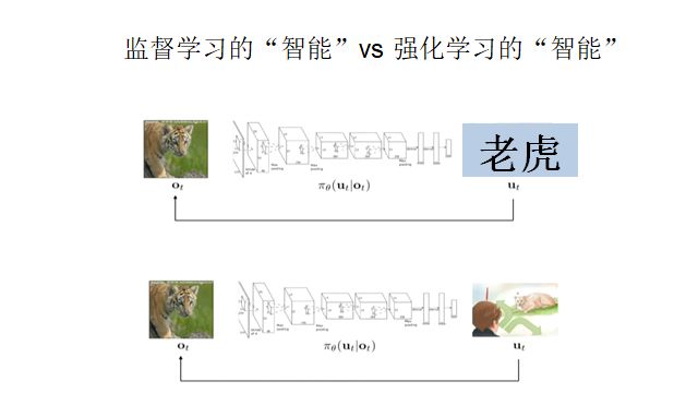
Before discussing RNNs, let’s first talk about reinforcement learning. Reinforcement learning is gaining increasing attention; its importance can be summarized with just one image. Imagine we are artificial agents, and we have the choice between reinforcement learning and supervised learning, but the tasks we undertake differ. When faced with a tiger, supervised learning would simply tell us the word ‘tiger’, but with reinforcement learning, we can decide whether to run away or fight. It is clear which option is more important because recognizing the tiger is meaningless if we do not decide whether to escape. Thus, reinforcement learning is needed to determine our actions.
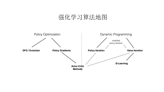
From an algorithmic perspective, reinforcement learning is an optimization problem for the future. The overarching algorithms can be summarized in the following diagram. There are two main schools of reinforcement learning: one is dynamic programming, and the other is policy gradient. Using the tiger example again, estimating the payoff function of fighting or not fighting over a 20-year period (for example, killing the tiger earns a reward, while being killed incurs a penalty) would be dynamic programming. In contrast, deciding to run or fight based on intuition and past experience would be the policy gradient method.
Dynamic programming requires iteration to learn; it is cumbersome but more precise. Direct learning is simpler but prone to getting stuck in local optima. To leverage the advantages of both methods, combining them yields the Actor-Critic method, which directly learns behaviors while evaluating the impact of those behaviors on future outcomes, thus informing the learning process.
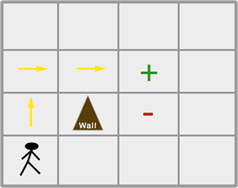
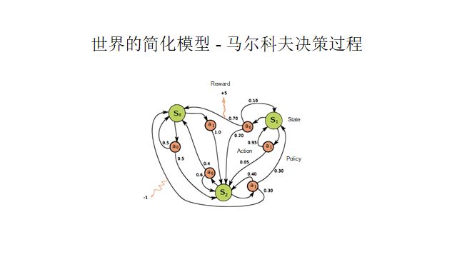
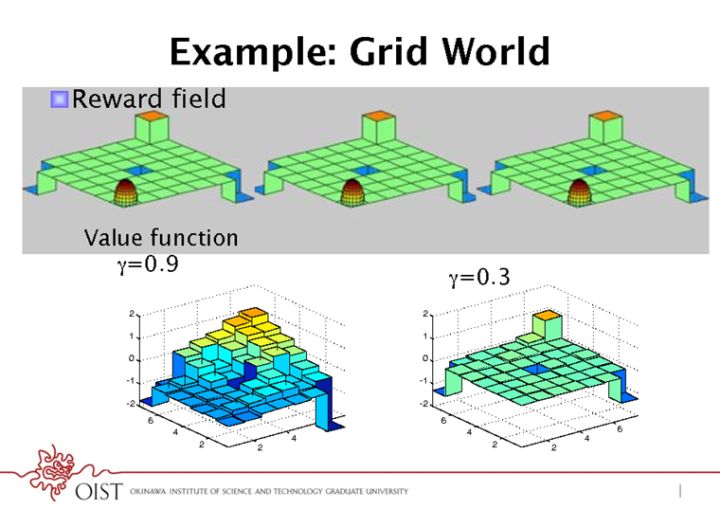
The success of reinforcement learning optimization algorithms began within the Markov decision framework. As long as a problem fits this framework (breaking the process into countless discrete moments, where the information at any moment is sufficient to decide future outcomes without historical information), it can be decomposed into four elements: state, action, reward, and policy. The state is the total information relevant to decision-making at each moment, the action is your decision, the reward is your immediate gain, and the policy is the correspondence from state to action. For example, in a grid maze (as shown in the diagram below), your state is your position, your action is moving up, down, left, or right, and your reward is the plus sign in the center. Each step in the process is only related to the previous step; at this moment, you have absolute information (your position), so it can be simplified into the Markov decision diagram framework shown below.
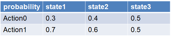
Only the policy is the target for optimization. The simplest tabular method for the policy is a table with states on one axis and actions on the other, where each cell contains the probability of taking a certain action in a given state.
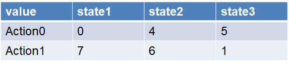
If you use the dynamic programming method mentioned earlier for optimization, you will also need another table called the Q-table, which similarly has states on one axis and actions on the other, but the contents of each corresponding cell are values, mathematically representing the expected future reward from a certain state-action pair. We iteratively learn and update this table.
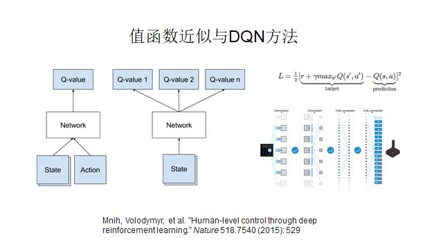
So where does deep reinforcement learning come from? In real life, there are too many states, such as the 3^361 states in Go, making the table method impractical. This naturally leads to the introduction of machine learning. Machine learning, especially neural networks, is fundamentally about function approximation or some form of interpolation. When the table becomes too large to fill, we replace it with a function and use neural networks to learn this function, which naturally introduces deep reinforcement learning. Through data, we can simulate the function, and with the function, we can solve the value function problem.
The DQN deep value function algorithm is the most basic deep reinforcement learning algorithm. The 2015 paper on Alpha-Go is based on value function methods, policy gradients, and Monte Carlo trees, combined with CNNs.
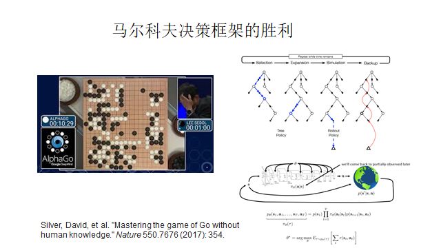
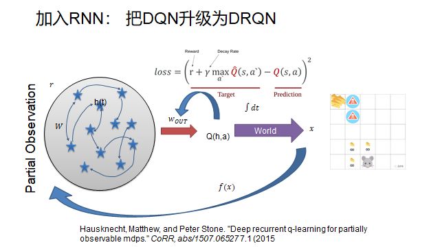
However, no matter how powerful Alpha-Go is, it cannot solve all problems, such as StarCraft, because the information in the current game screen is insufficient for decision-making. The information required for decision-making is not all presented in one screen, which creates an opportunity for our other protagonist, RNN.
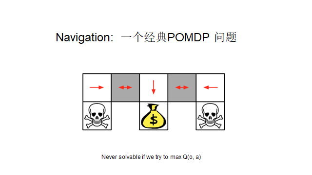
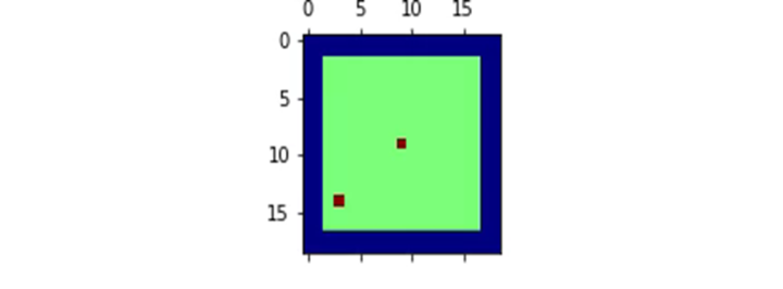
Let’s illustrate with a minimal example, still using the grid problem. The skull indicates danger, and we want to reach the rewarding location. I will make a small modification that changes the entire nature of the problem; the previous Markov decision condition was that the current state contained all the information necessary for decision-making, and in the grid problem, this information is the position coordinates. If I do not have this position information and instead rely on perceptual information, for example, I can only sense what is in the two adjacent squares (the skull or the coin in the diagram below).
Note that if we are in the gray square area in the diagram below (with one on each side), the situations in the two adjacent squares are identical (white). This means I cannot determine whether I am in the left or right gray square, leading to an inability to decide on the correct action (the correct decisions for left and right are opposite! One left and one right, but I cannot tell which is which!).
Real-life organisms live in environments of incomplete information every day, surrounded by situations like the gray squares in the diagram above. They must still learn the correct behaviors. So how do they solve this problem?
There are mainly three methods: one is the policy gradient method, where, despite incomplete state and information, we can use probabilistic methods to learn. When unsure whether to go left or right, we can take a random step, giving a 50% chance of ultimately receiving the desired reward (like a donkey in the desert; it must choose a direction to walk or it will die of thirst). This method utilizes direct learning of the policy function, i.e., Policy Gradient, to solve the problem. However, this method is relatively inefficient; if time is limited, it could lead to failure.
The second method is to introduce memory. With memory, you can essentially piece together information from different time points into a whole, providing you with more information than before. In the grid example above, if you know whether you came from the left or right boundary in the previous step, the problem can be resolved. The final method is to build an accurate world model. While your information is incomplete, you can use your brain to model the world, transforming an incomplete world into a complete one in your mind.
The introduction of memory naturally leads us to RNNs, which mimic the principles of biological working memory, storing information in memory to inform decision-making.
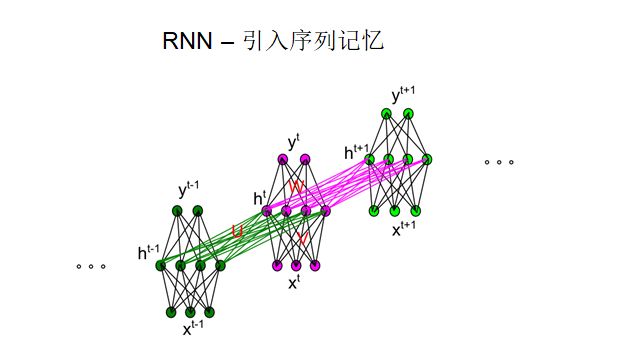
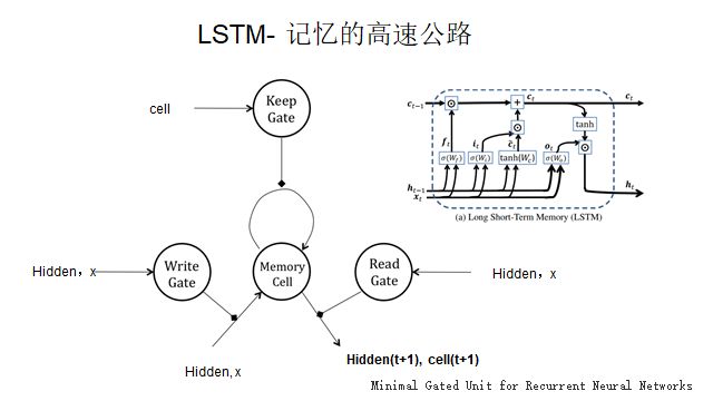
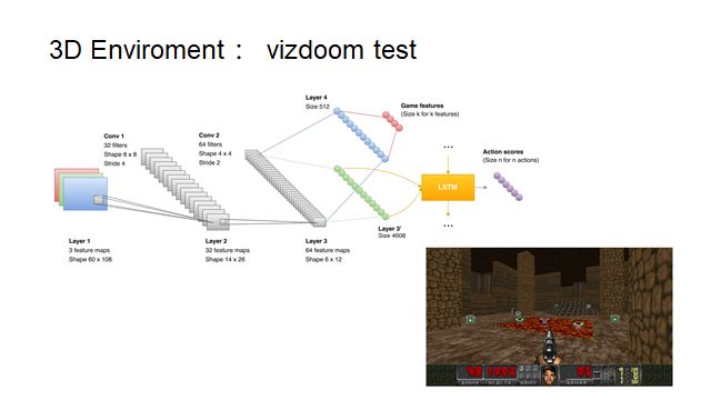
The RNN network structure is not vastly different from that of feedforward neural networks; it simply adds a time transition matrix, connecting the current hidden state to the next hidden state. This connection effectively transmits current information to the next moment, containing memory in this process. We can iterate past information into the future, thus embedding many past moments into the neural network cells, akin to biological working memory. LSTM adds a memory cell layer on top of RNN, allowing for the separation of past and current information, where past information runs directly in the cell and current decisions operate in the hidden state. With RNNs, DQN evolves into DRQN, enabling navigation through very complex environments.
The diagram below depicts a two-dimensional maze where only the states of adjacent squares are visible, representing an expanded version of the previously described problem (akin to searching for water in a desert, where only the surrounding information is visible). What we need to do is navigate through complex situations to find the target, which is a navigation problem. The red dot in the lower left corner indicates the starting position, while the center red dot is the target. The behavior learned is that the agent will directly move to the wall to gain information about its position, and then from there head towards the target, simulating the process of spatial search. In this process, RNN stitches together information from different time points into a whole.
While RNNs have this capability, they can still be perplexed when the space becomes complex, such as in a hotel with many rooms. At this point, stronger spatial representation abilities are required. This can also be induced through learning; the usual approach is to incorporate elements of supervised learning, such as learning to predict your position in space. In this process, the ability to simulate space will automatically emerge in the dynamical structure of RNNs.
Supervised learning signals are abundant and have clear objectives; they can predict where to go and how far from the reward, effectively giving reinforcement learning wings.
Once we introduce supervised learning, we essentially achieve the third strategy mentioned earlier: introducing a world model, albeit through a step-by-step process rather than all at once.
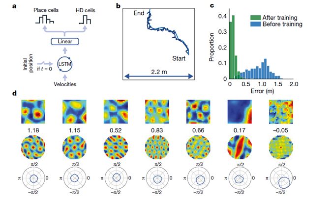
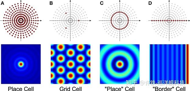
A paper published in Nature further advanced this concept. It also employs supervised learning but induces RNN (LSTM) to form a new structure based on fundamental learning. Remarkably, this structure closely resembles the grid cells found in the brains of mice. These grid cells represent space as a network composed of many hexagons, where each cell is sensitive to the endpoint positions of the hexagonal network, and different cells respond to different spatial periods (grid edge lengths).
The essence of this method is to establish a general model of space. Clearly, your brain does not create entirely distinct and isolated neural representations for Beijing, Shanghai, or Tianjin; there must be a spatial language that supports all spatial concepts, and the expression at the most fundamental level remains unchanged as you move from one place to another. This can be viewed as a model on top of another model, which is precisely what grid cells represent. Each grid cell corresponds to a hexagonal network of a different spatial period, and by combining these hexagonal networks, we can easily obtain representations of relative spatial positions (similar to a Fourier transform, where each grid cell is a component of the Fourier transform, read by downstream position cells).
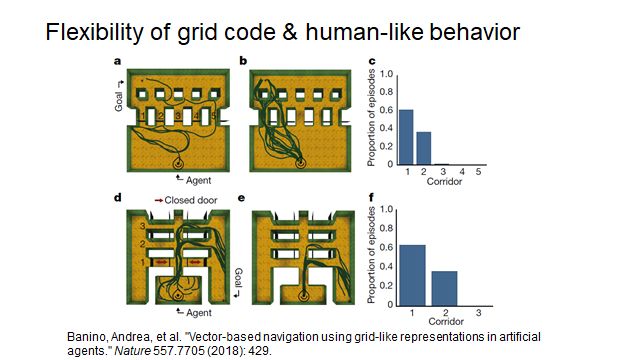
With this network of cells, there will be a stronger ability to navigate in space. A hallmark of this ability is that it can find shortcuts in complex spaces. If the path changes (for example, if a door is blocked), it will seek a suboptimal target, indicating a form of dynamic planning capability, or intelligence in spatial navigation. By adding appropriate supervised learning on top of RNNs, we can produce structures similar to biological cells, thus acquiring spatial expression capabilities.
In conclusion, we can summarize the potential of RNNs in reinforcement learning: RNNs, as dynamic systems, inherently express the connections between the past, present, and future, which can be viewed as partial or complete world models. Reinforcement learning, as an optimization of future rewards, can be seen as a sequential decision-making problem. The more thoroughly you understand the past, present, and future of the system, the stronger your decision-making ability. Hence, RNNs inherently have a certain compatibility with reinforcement learning. RNNs’ dynamic systems can be said to express partial or complete world models, making them not only powerful tools for solving local Markov problems but also bridges in both model-free and model-based reinforcement learning.
Related Reading
Iron Brother’s Long Article: An Introduction to Neural Navigation – Discussing DeepMind’s Latest Article
From Q-learning’s Mini Games to AlphaGo Technology
For a deeper understanding, please refer to the following articles:
Bakker B. Reinforcement learning with long short-term memory[C]//Advances in neural information processing systems. 2002
The earliest attempts to introduce RNN into reinforcement learning primarily emphasized that RNNs can solve POMDPs.
Hausknecht, Matthew, and Peter Stone. “Deep recurrent q-learning for partially observable mdps.” CoRR, abs/1507.06527 7.1 (2015).
This article follows up on the 2002 paper, emphasizing that information-deficient Atari Games can achieve performance breakthroughs through RNNs (LSTM).
Mirowski, Piotr, et al. “Learning to navigate in complex environments.” arXiv preprint arXiv:1611.03673 (2016)
Noteworthy literature in navigation, introducing how to further incorporate supervised learning in deep reinforcement learning with RNNs (LSTM) to achieve performance breakthroughs.
Wang J X, Kurth-Nelson Z, Tirumala D, et al. Learning to reinforcement learn[J]. arXiv preprint arXiv:1611.05763, 2016.
A niche piece, introducing a form of reinforcement meta-learning capability based on RNNs, akin to a generalization ability.
Banino, Andrea, et al. “Vector-based navigation using grid-like representations in artificial agents.” Nature 557.7705 (2018): 429.
The latest Nature article introduces the ability of RNNs (LSTM) to generate spatial grid cells through supervised learning.
Author: Xu Tie, WeChat: ironcruiser
Master's in Physics from École Normale Supérieure in Paris, PhD in Computational Neuroscience from Technion-Israel Institute of Technology (a cradle for 85% of Israel's tech entrepreneurs, renowned for computer science), founder of Cruiser Technology Ltd., previously worked for one year at the Center for Nonlinear Science at Hong Kong Baptist University, a good comrade of Principal Wanmen Tong.

Xu Tie's book "Machine Learning and Complex Systems" views machine learning from a physics perspective and is now officially on sale. At the same time, Xu Tie has launched two online courses on the principles of machine learning and deep learning at Wanmen University, with a live online course on reinforcement learning set to begin in September. Interested parties can click the QR code in the image below for inquiries.