
Author: Huang Tianyuan, currently a PhD student at Fudan University, with research involving text mining, social network analysis, and machine learning. I hope to share learning experiences and promote the application of R language in the industry.
Email: [email protected]
XGBoost is currently the best predictive solution based on tree models, and is worth exploring and practicing. Here, I will provide a brief practical operation and introduction based on DALEX_and_xgboost (for related content, click Read Original).
# Regression Model
## Data Loading
We will use the wine function from the breakDown package for modeling.
“`{r}
library(“breakDown”)
head(wine)
“`
## Model Building
When modeling with the xgboost package, all variables must be converted to numeric, and the best approach is to use the built-in data type of the xgboost package (constructed using `xgb.DMatrix`). First, let’s construct this matrix:
“`{r}
library(“xgboost”)
model_matrix_train <- model.matrix(quality ~ . – 1, wine)
data_train <- xgb.DMatrix(model_matrix_train, label = wine$quality)
“`
Here, the `model.matrix` function is generally used to flatten factor variables into numeric, but since our dataset has no factor variables, we simply extracted the response variable and converted it into matrix type. Next, we will set the necessary parameters and start modeling.
“`{r}
param <- list(max_depth = 2, eta = 1, silent = 1, nthread = 2,
objective = “reg:linear”)
wine_xgb_model <- xgb.train(param, data_train, nrounds = 50)
wine_xgb_model
“`
We are using a linear model; please refer to the official website
## Model Interpretation
Simply use the explain function from the DALEX package.
“`{r}
library(“DALEX”)
explainer_xgb <- explain(wine_xgb_model,
data = model_matrix_train,
y = wine$quality,
label = “xgboost”)
explainer_xgb
“`
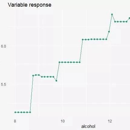
## Univariate Analysis
How does the quality of wine change with the alcohol content?
“`{r}
sv_xgb_satisfaction_level <- variable_response(explainer_xgb,
variable = “alcohol”,
type = “pdp”)
head(sv_xgb_satisfaction_level)
plot(sv_xgb_satisfaction_level)
“`
## Contribution of Different Variables in a Single Prediction
Although the model summarizes the overall data, each variable’s contribution to the final prediction varies for different individuals. Let’s take the first sample and try it out.
“`{r}
nobs <- model_matrix_train[1, , drop = FALSE]
sp_xgb <- prediction_breakdown(explainer_xgb,
observation = nobs)
head(sp_xgb)
plot(sp_xgb)
“`
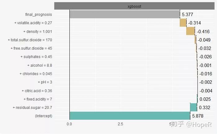
From this experiment, we can see that fixed.acidity and residual.sugar are considered to have a positive effect on this prediction, while volatile.acidity and density have the opposite effect.
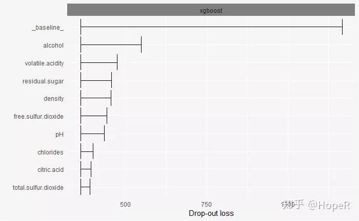
## Variable Importance
“`{r}
vd_xgb <- variable_importance(explainer_xgb, type = “raw”)
head(vd_xgb)
plot(vd_xgb)
“`
# Classification Model
## Data Loading
We will explore a dataset for predicting employee turnover.
“`{r}
library(“breakDown”)
head(HR_data)
“`
## Model Building
The process is basically the same as above, so I won’t elaborate. It is worth noting that this dataset contains factor variables, so using model.matrix is very appropriate. In addition, the formula `left ~ . – 1` indicates that we are subtracting the intercept; if you don’t understand, you can try without subtracting. Since the response variable has only two types, we will use logistic regression, with AUC as the evaluation standard.
“`{r}
library(“xgboost”)
model_matrix_train <- model.matrix(left ~ . – 1, HR_data)
data_train <- xgb.DMatrix(model_matrix_train, label = HR_data$left)
param <- list(max_depth = 2, eta = 1, silent = 1, nthread = 2,
objective = “binary:logistic”, eval_metric = “auc”)
HR_xgb_model <- xgb.train(param, data_train, nrounds = 50)
HR_xgb_model
“`
## Model Interpretation
DALEX can only handle numeric response variables, so we need to set the link function and prediction function.
“`{r}
library(“DALEX”)
predict_logit <- function(model, x) {
raw_x <- predict(model, x)
exp(raw_x)/(1 + exp(raw_x)) # Although the official documentation includes this, is it really necessary? The predicted values themselves are probability values.
}
logit <- function(x) exp(x)/(1+exp(x))
“`
Let’s take a look at the function’s functionality. The predict_logit function takes a model and data x (although the type is not defined, we can infer that it is a new dataset), predicts new data based on the model, and then transforms the predicted values (link function). The logit is the format of the link function.
Next, we will use the function for interpretation.
“`{r}
explainer_xgb <- explain(HR_xgb_model,
data = model_matrix_train,
y = HR_data$left,
predict_function = predict_logit,
link = logit,
label = “xgboost”)
explainer_xgb
“`
# Univariate Analysis
“`{r}
sv_xgb_satisfaction_level <- variable_response(explainer_xgb,
variable = “satisfaction_level”,
type = “pdp”)
head(sv_xgb_satisfaction_level)
plot(sv_xgb_satisfaction_level)
“`
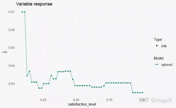
As satisfaction increases, the probability of turnover decreases.
# Single Sample Prediction
“`{r}
nobs <- model_matrix_train[1, , drop = FALSE]
sp_xgb <- prediction_breakdown(explainer_xgb,
observation = nobs)
head(sp_xgb)
plot(sp_xgb)
“`
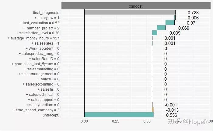
For this employee, the last evaluation has the greatest contribution of this variable.
## Variable Importance
“`{r}
vd_xgb <- variable_importance(explainer_xgb, type = “raw”)
head(vd_xgb)
plot(vd_xgb)
“`
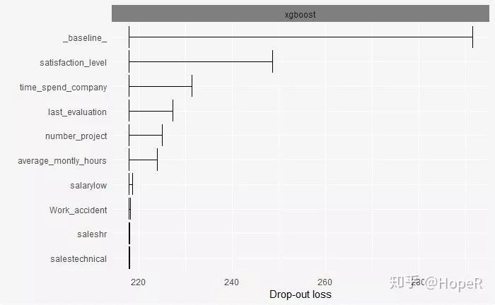
Employee satisfaction is the variable that best reflects turnover rates.
——————————————
Past Highlights:
-
Today, I changed my name!
-
Big Bowl Wide Noodles VS Lawyer Letter Warning, Sentiment Analysis of Kris Wu’s Self-Mocking Fan Engagement!
-
Selected | Recommended R New Packages in March 2019