Selected from Kdnuggets
Author:Lars Hulstaert
Translated by Machine Heart
Contributors: Yan Qi, Li Zenan
This article is aimed at slightly experienced machine learning developers. Lars Hulstaert from Microsoft introduces several objective functions for training neural networks.
Introduction
The motivation for writing this article has three aspects:
-
First, there are many articles introducing optimization methods, such as how to optimize stochastic gradient descent or propose a variant of that method, but few explain how to construct the objective function of a neural network. They answer questions like: Why are mean squared error (MSE) and cross-entropy loss used as objective functions for regression and classification tasks, respectively? Why does adding a regularization term make sense? Therefore, the significance of writing this blog post is that by examining the objective functions, people can understand how neural networks work and why they may fail in other domains.
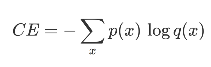
In classification tasks (in supervised learning), the cross-entropy loss between the correct label p (ground truth) and the network output q.
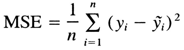
In regression tasks (in supervised learning), the mean squared error between the correct label y and the network output y_tilde.
-
Second, neural networks are notorious for making incorrect probability predictions, and they also struggle with adversarial examples (a special type of input data specifically designed by researchers to make neural networks make incorrect predictions). In summary, neural networks are often overly confident, even when they make mistakes. This issue cannot be ignored in real environments; for example, an autonomous vehicle must ensure it can make correct decisions while traveling at 145 km/h. Therefore, if we are to apply deep learning on a large scale, we must not only recognize its advantages but also understand its shortcomings.
-
I have always wanted to understand why neural networks can be explained from a probabilistic perspective and why they are suitable as a general framework for machine learning models. People like to discuss the output of the network as probabilities. So, is there a connection between the probabilistic interpretation of neural networks and their objective functions?
The inspiration for writing this article came from the author’s research on Bayesian neural networks during his time working with his friend Brian Trippe at the Cambridge University Computational and Biological Learning Lab. The author highly recommends readers check out Brian’s paper on variational inference in neural networks titled “Complex Uncertainty in Machine Learning: Bayesian Modeling for Conditional Density Estimation and Synaptic Plasticity”.
Supervised Learning
In supervised learning problems, we generally have a dataset D, where x is a sample and y is the sample label. We represent the sample as (x, y), and what we need to do is model the conditional probability distribution P(y | x, θ).
For example, in an image classification task, x represents an image and y represents the corresponding image label. P(y | x, θ) indicates the probability of label y given the image x and a model defined by parameters θ.
The model established by this method is called a discriminative model. In discriminative or conditional models, the parameters θ that define the conditional probability distribution function P(y|x, θ) are derived from the training set.
Based on the observed data x (input data or features), the model outputs a probability distribution, which will then be used to predict the label y (class or true value). Different machine learning models require different parameters for prediction. For linear models (e.g., logistic regression, defined by a series of weights equal to the number of features) and nonlinear models (e.g., neural networks, defined by a series of weights in each of its layers), both types of models can be approximated as conditional probability distributions.
For typical classification problems, the (learnable) parameters θ are used to define a mapping from x to a categorical distribution (based on different labels). A discriminative model outputs probabilities for N (where N is the number of classes). Each x belongs to a single class, but the model’s uncertainty is reflected in a distribution output over the classes. Generally, the class with the highest probability is chosen when making a decision.
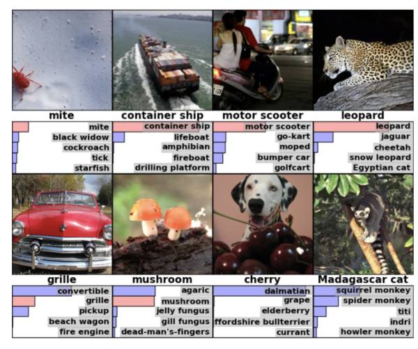
In image classification, the network outputs a categorical distribution based on the image class. The above figure describes the top five classes in a test image (filtered by probability size).
We note that a discriminative regression model often outputs only a single predicted value rather than a distribution based on all true values. This is different from a discriminative classification model, which outputs a distribution based on possible classes. So does this mean that the discriminative model collapses for regression tasks? Shouldn’t the model’s output tell us which regression values are more likely than others?
To say that a discriminative regression model has only one output can be misleading; in fact, the output of a regression model is related to a well-known probability distribution: the Gaussian distribution. It turns out that the output of a discriminative regression model represents the mean of a Gaussian distribution (a Gaussian distribution is completely defined by a mean and a standard deviation). With this information, you can determine the similarity of each true value given an input *x*.
Typically, only the mean of this distribution is modeled, while the standard deviation of the Gaussian distribution is either not modeled or kept constant across all x. Therefore, in the discriminative regression model, θ defines a mapping from x to the mean of the Gaussian distribution (from which y is sampled). Essentially, whenever a decision needs to be made, we select the mean, as the model can express which x is uncertain by increasing the standard deviation.
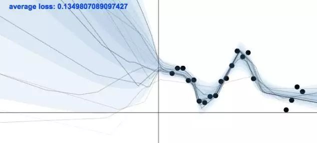
When there is no training data, a model needs to remain uncertain; conversely, when there is training data, the model needs to become certain. The above figure illustrates such a model, with the image sourced from Yarin Gal’s blog.
In regression problems, other probabilistic models (such as Gaussian processes) perform much better in modeling uncertainty. Because when trying to model both the mean and the standard deviation simultaneously, discriminative regression models tend to be overly confident.
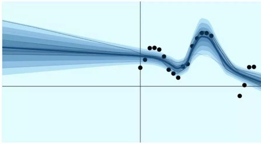
Gaussian processes can quantify uncertainty by accurately modeling the standard deviation. Its only drawback is that Gaussian processes do not scale well to large datasets. In the figure below, you can see that the GP model has a small confidence interval around regions with a lot of data. In areas with few data points, the confidence interval becomes large.
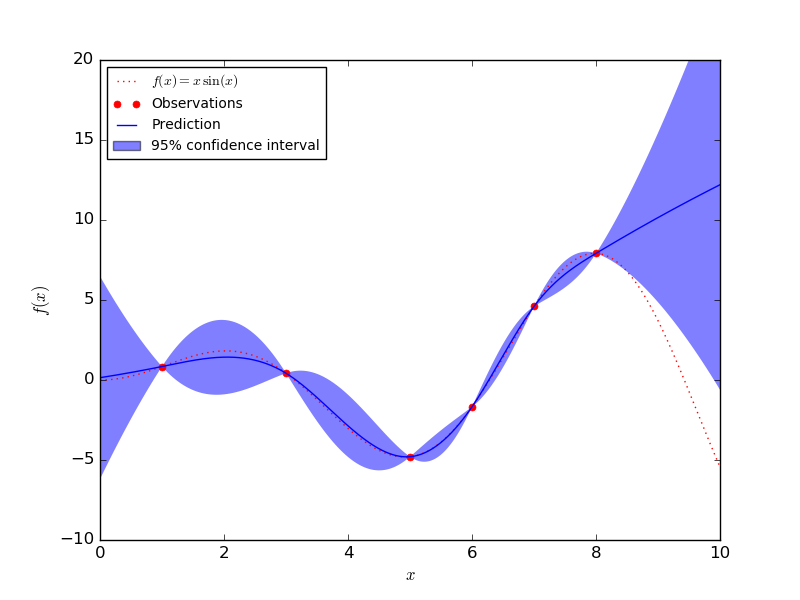
The GP model is certain at data points but uncertain elsewhere (image from Sklearn).
By training on the training set, the discriminative model can learn features in the data (representing a class or true value). If a model can assign high probabilities to correctly labeled sample classes or close to the true value mean in the test set, we say the model performs well.
Linking Neural Networks
When using neural networks for classification or regression tasks, the modeling of the aforementioned parameter distributions (categorical distribution and Gaussian distribution) is accomplished through the neural network.
This becomes clearer when we want to determine the maximum likelihood estimation (MLE) of the neural network parameters θ. MLE is equivalent to finding the parameters θ that maximize the likelihood (or equivalently, the log-likelihood) of the training dataset. More specifically, the expression in the figure below is maximized:
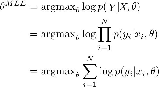
When p(Y | X, θ) is determined by the model, it represents the probability of the true labels in the training data. If p(Y | X, θ) is close to 1, it means the model can determine the correct labels/mean in the training set. Given a training dataset (X,Y) composed of N observation pairs, the likelihood of the training data can be rewritten as the sum of the log probabilities.
In the cases of classification and regression, p(y|x, θ) as a posterior probability of (x, y) can be rewritten into categorical and Gaussian distributions. In optimizing neural networks, the objective is to change the parameters, specifically: for a series of inputs X, the correct parameters for the probability distribution Y can be obtained from the output (regression values or classes). Generally, this can be achieved through gradient descent and its variants. Therefore, to obtain an MLE estimate, our goal is to optimize the model output concerning the true output:
-
Maximizing the log value of a categorical distribution is equivalent to minimizing the cross-entropy between the true distribution and its approximate distribution.
-
Maximizing the log value of a Gaussian distribution is equivalent to minimizing the mean squared error between the true mean and its approximate mean.
Thus, the expressions in the aforementioned image can be rewritten as cross-entropy loss and mean squared error, as well as the objective functions for neural networks in classification and regression.
Compared to more traditional probabilistic models, the nonlinear functions learned by neural networks from input data to probabilities or means are difficult to interpret. Although this is a significant drawback of neural networks, their ability to model a vast range of complex functions brings immense benefits. From this part of the derived discussion, it is evident that the objective functions of neural networks (formed in the process of determining parameters via MLE likelihood) can be interpreted probabilistically.
An interesting interpretation of neural networks relates to their relationship with general linear models (linear regression, logistic regression). Compared to selecting linear combinations of features (as done in GLMs), neural networks produce highly nonlinear combinations of features.
Maximum A Posteriori (MAP)
But if neural networks can be interpreted as probabilistic models, why is the quality of the probability predictions they give so poor, and why can’t they handle adversarial examples? Why do they require so much data?
When choosing a good function approximator, I tend to select different models (logistic regression, neural networks, etc.) depending on the search space. When faced with an enormous search space, which means you can flexibly model posterior probabilities, it still comes at a cost. For example, neural networks have been shown to be universal function approximators. This means that as long as there are enough parameters, they can model any function. However, to ensure that the function is well-calibrated across the entire data space, a massive dataset is essential.
Typically, a standard neural network uses MLE for optimization, and it is important to understand this. Optimizing with MLE can lead to overfitting, so the model requires a large amount of data to mitigate the overfitting issue. The goal of machine learning is not to find a model that explains the training data best. We need to find a model that has good generalization capabilities on data outside the training set.
Here, the Maximum A Posteriori (MAP) method is an effective alternative, often used when probabilistic models encounter overfitting issues. So what does MAP mean in the context of neural networks? What impact does it have on the objective function?
Similar to MLE, MAP can also be rewritten as an objective function in the context of neural networks. Essentially, using MAP means you are maximizing the probability of a series of parameters θ (given data, assuming a prior probability distribution on θ):
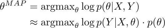
When using MLE, we only consider the first element of the equation (to what extent the model explains the training data). When using MAP, it is also important for the model to satisfy the prior probability to reduce overfitting (to what extent θ satisfies the prior probability).
Using a Gaussian prior with a mean of 0 on θ is equivalent to applying L2 regularization to the objective function (ensuring many small weights), while using a Laplace prior on θ is equivalent to applying L1 regularization to the objective function (ensuring many weights are zero).
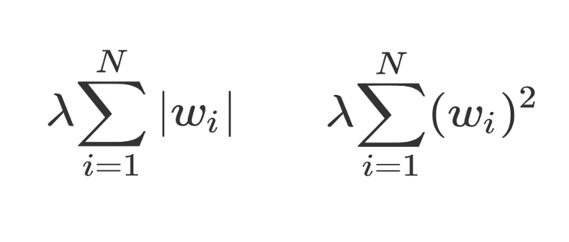
On the left is L1 regularization, and on the right is L2 regularization.
A Fully Bayesian Approach
In both MLE and MAP cases, only one model is used (it has only one set of parameters). This is especially true for complex data like images, where the issue of specific regions in the data space not being covered is unlikely to arise. The model’s output in these areas is determined by the model’s random initialization and training process, and the model will give very low probability estimates for points outside the coverage area of the data space.
Although MAP ensures that the model does not overfit too much in these areas, it still makes the model overly confident. In a fully Bayesian approach, we address this issue by averaging over multiple models, which can yield better uncertainty predictions. Our goal is to model a distribution of parameters rather than just a single set of parameters. If all models (with different parameter settings) give different predictions outside the coverage area, it means there is significant uncertainty in that region. By averaging these models, we ultimately obtain a model that is uncertain in those areas, which is exactly what we want.
Original link:https://www.kdnuggets.com/2017/11/understanding-objective-functions-neural-networks.html
This article is translated by Machine Heart, please contact this public account for authorization to reprint.
✄————————————————
Join Machine Heart (full-time reporter/intern): [email protected]
Submissions or inquiries: [email protected]
Advertising & Business Cooperation: [email protected]