Understanding Neural Network Architectures Through 25 Images

As new neural network architectures emerge constantly, it is quite challenging to document all neural networks. Understanding all the networks represented by these abbreviations (DCIGN, IiLSTM, DCGAN, etc.) can be daunting at first.

The table below includes most commonly used models (mostly neural networks, along with some other models). Although these architectures are novel and unique, when I began to visualize their results, the underlying relationships of each architecture became clear.

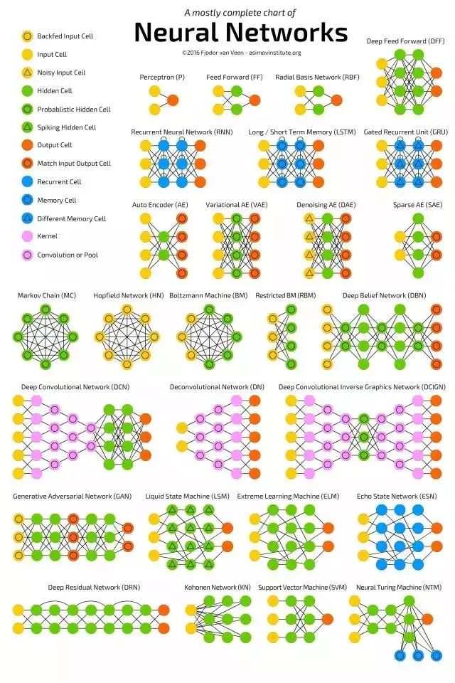
Clearly, these node diagrams do not reveal the internal workings of each model. For example, the node diagrams for Variational Autoencoders (VAE) and Autoencoders (AE) look the same, but their training processes are fundamentally different, and the use cases of the models post-training are also quite distinct. VAE acts as a generator, used to inject noise into samples, while AE simply maps the inputs it receives to the nearest training samples in its ‘memory’! This article does not delve into the internal workings of each different architecture.

Although most abbreviations have been widely accepted, some conflicts may arise. For example, RNN typically refers to Recurrent Neural Networks, but it can also refer to Recursive Neural Networks, and in many contexts, it just generically refers to various recurrent architectures (including LSTM, GRU, and even bidirectional variants). AE is similar; VAE and DAE are often simply referred to as AE. Additionally, the same model can have different suffixes for the number of N’s. The same model can be called Convolutional Neural Network or Convolutional Network, leading to the abbreviations CNN or CN.

It is almost impossible to treat this article as a complete list of neural networks, as new architectures are continually being invented, and even when new architectures are released, finding them can be challenging. Therefore, this article may provide some insights into the world of AI but is by no means exhaustive; especially if you are reading this long after its publication.

For each architecture depicted above, this article provides a very brief description. If you are very familiar with certain architectures, you may find some of this useful.

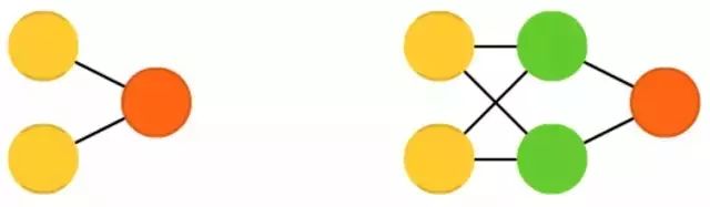
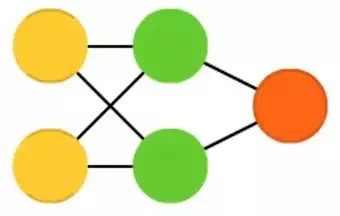
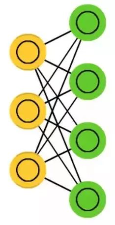
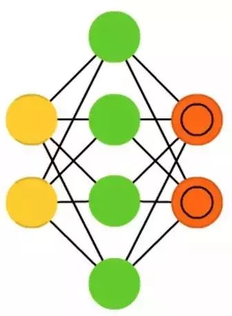
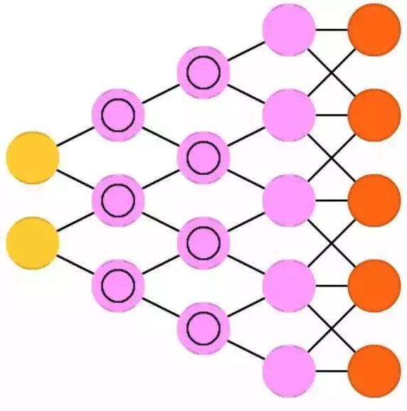
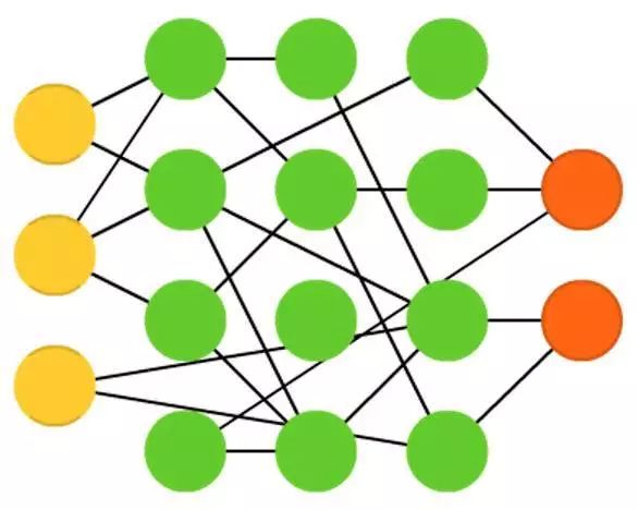
Perceptron (P, left) and Feedforward Neural Networks (FF or FFNN, right) are very intuitive; they take information from the front end as input and produce output from the back end. Neural networks are typically described as having layers (input, hidden, or output layers), with each layer consisting of parallel units. Generally, there are no connections within the same layer, and two adjacent layers are fully connected (each neuron in one layer connects to every neuron in the other layer).

The simplest practical network has two input units and one output unit, used to establish logical models (used for determining yes or no). FFNN are typically trained using backpropagation, with datasets made up of paired input and output results (this is called supervised learning). We provide it with input and let the network fill in the output. The error in backpropagation is typically some variation of the difference between the filled output and the actual output (such as MSE or merely linear difference). Given that the network has enough hidden neurons, it can theoretically always model the relationship between input and output. In practice, their applications are quite limited, and they are often combined with other networks to form new networks.

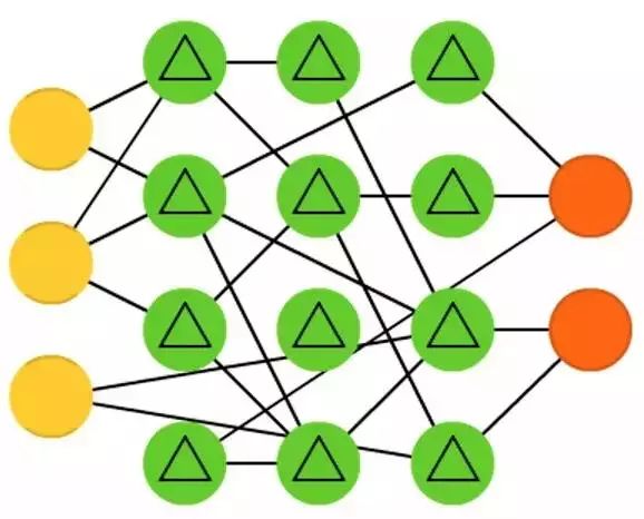
Radial Basis Function (RBF) networks are essentially FFNN networks that use radial basis functions as activation functions. However, RBFNN has its distinct use cases that differ from FFNN (due to the time of invention, most other activation function-based FFNNs do not have their own names).

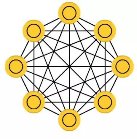
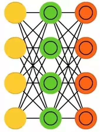
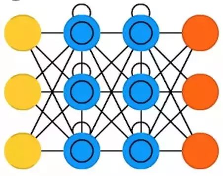
Hopfield Networks (HN) have each neuron connected to other neurons; its structure resembles a plate of completely entangled spaghetti. Each node inputs data before training and then hides and outputs during training. The network is trained by setting the values of neurons to desired patterns, after which the weights remain unchanged. Once one or more patterns have been trained, the network will always converge to one of the learned patterns, as the network is stable in this state. It is important to note that HN does not always maintain consistency with the ideal state. The stability of the network is partly due to the overall ‘energy’ or ‘temperature’ gradually decreasing during training.

Each neuron has an activation threshold that changes with temperature; once the sum of inputs exceeds this threshold, the neuron will take one of two states (usually -1 or 1, sometimes 0 or 1). The updating of the network can occur synchronously or sequentially; the latter is more common. When updating the network sequentially, a fair random sequence is generated, and each unit is updated in a prescribed order. Thus, when each unit has been updated and no longer changes, you can determine that the network is stable (no longer converging). These networks are also known as associative memory, as they will converge to the state most similar to the input; when humans see half a table, we imagine the other half of the table; if the input is half noise and half table, HN will converge to a table.

Markov Chains (MC or Discrete-Time Markov Chains, DTMC) are predecessors of BM and HN. It can be understood as follows: from my current node, the probability of going to any neighboring node is random, meaning the node you ultimately choose depends entirely on the current node you are in, regardless of the nodes you were in the past. Although this is not a true neural network, it resembles a neural network and forms the theoretical basis for BM and HNs. Like BM, RBM, and HN, MC is not always considered a neural network. Additionally, Markov chains are not always fully connected.

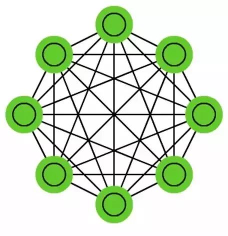
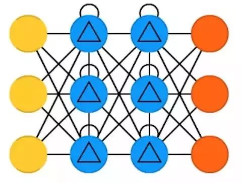
Boltzmann Machines (BM) are quite similar to HN, with the distinction that only some neurons are designated as input neurons while the others remain ‘hidden’. The input neurons become output neurons at the end of a complete network update. It starts with random weights and trains the model either through backpropagation learning or by contrastive divergence (a Markov chain used to determine the gradient between two information gains).

Compared to HN, most of the neurons in BM have binary activation patterns. Trained by MC, BM is a random network. The training and operation processes of BM are very similar to HN: setting input neurons to certain clamped values to activate the network. While the released nodes can take any value, this leads to multiple iterations between the input and hidden layers. Activation is controlled by a global threshold. This gradual reduction of global error leads the network to eventually reach equilibrium.

Restricted Boltzmann Machines (RBM) are very similar to BM and also resemble HN. The main difference between BM and RBM is that RBM has better usability because it is more constrained. RBM does not connect every neuron to every other neuron but connects each group of neurons to every other group, so there are no input neurons directly connected to other input neurons, nor hidden layers directly connected to hidden layers. RBM can be trained like FFNN, rather than propagating data forward and then backpropagating.

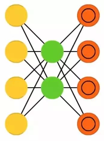
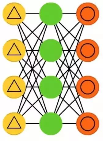
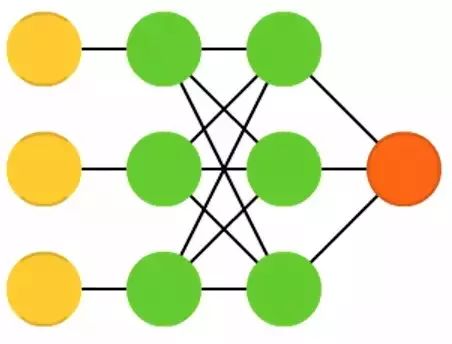
Autoencoders (AE) are somewhat similar to Feedforward Neural Networks (FFNN). Rather than being a completely different network structure, it is a different application of a feedforward neural network. The basic idea of an autoencoder is to automatically encode information (like compression, rather than encryption). Hence the name. The entire network is funnel-shaped: its hidden layer units are always fewer than those in the input and output layers.

Autoencoders are always symmetric about the central layer (the central layer being one or two depending on the number of layers in the network: if odd, symmetric about the middle layer; if even, symmetric about the two middle layers). The smallest hidden layer is always at the central layer, which is also where the information is most compressed (called the bottleneck of the network). The portion from the input layer to the central layer is called the encoding part, and from the central layer to the output layer is called the decoding part; the central layer is called the code. The autoencoder can be trained using backpropagation, inputting data into the network and setting the error as the difference between the input data and the output data of the network. The weights of the autoencoder are also symmetric, meaning the encoding and decoding weights are the same.

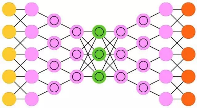
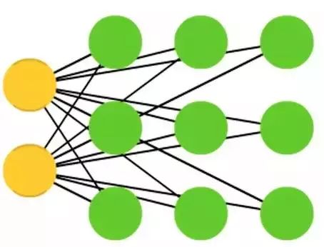
Sparse Autoencoders (SAE) are somewhat opposite to autoencoders. Rather than training a network to represent a bunch of information in a lower-dimensional space and nodes, here we try to encode information in a higher-dimensional space. Thus, in the central layer, the network expands rather than converges. This type of network can be used to extract features from a dataset. If we train sparse autoencoders using the same method as training standard autoencoders, we will almost always end up with a completely useless identity network (i.e., whatever input, the network outputs the same, without any transformation or decomposition).

To avoid this, a sparsity constraint is added during the feedback input process. This sparsity constraint can take the form of threshold filtering, meaning only specific errors can backpropagate and be trained, while other errors are considered irrelevant to training and set to zero. To some extent, this is similar to spiking neural networks: not all neurons are activated at every moment (which has some biological rationale).

Variational Autoencoders (VAE) share the same network structure as autoencoders but learn some other things: the approximate probability distribution of input samples. This is more similar to Boltzmann Machines (BM) and Restricted Boltzmann Machines (RBM). However, they rely on Bayesian mathematics, which involves probabilistic inference and independence, as well as reparameterization techniques to obtain different representations.

The probabilistic inference and independence part has intuitive meaning, but they rely on complex mathematical knowledge. The basic principle is as follows: consider the influences. If something happens in one place and something else happens elsewhere, they may not be related. If they are not related, this should be taken into account during the error backpropagation. This approach is useful because neural networks are large graphs (to some extent), so as you go deeper into the network layers, you can exclude the influence of some nodes on others.

Denoising Autoencoders (DAE) are a type of autoencoder. In denoising autoencoders, we do not input raw data, but rather data with noise (like making the image more grainy). However, we compute the error in the same way as before. Thus, the output of the network is compared to the original input data without noise. This encourages the network to learn not just the details but also broader features. Since features may vary with noise, the features learned by the standard network are usually incorrect.

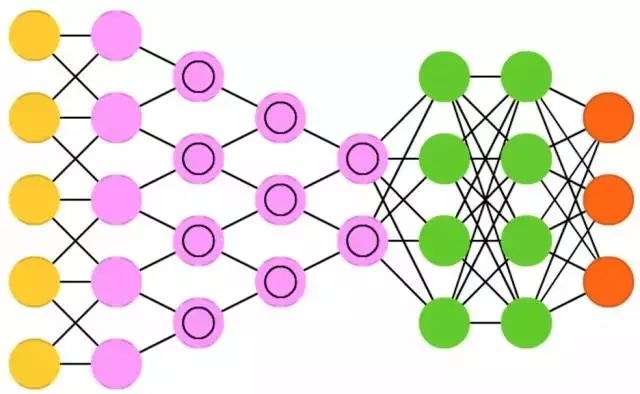
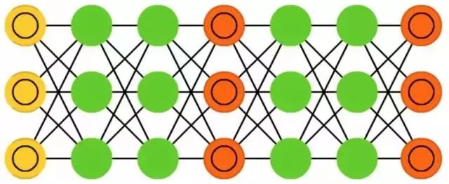
Deep Belief Networks (DBN) are stacked structures of Restricted Boltzmann Machines or Variational Autoencoders. These networks have been shown to be effectively trainable. Each autoencoder or Boltzmann Machine only needs to learn to encode the previous network. This technique is also referred to as greedy training. Greedy refers to seeking only local optimal solutions in a descending process, which may not be the global optimal solution.

Deep Belief Networks can be trained through contrastive divergence or backpropagation, and like conventional Restricted Boltzmann Machines or Variational Autoencoders, they learn to represent data as probabilistic models. Once the model has been trained through unsupervised learning or converged to a (more) stable state, it can be used to generate new data. If trained using contrastive divergence, it can even classify existing data, as neurons are taught to look for different features.

Convolutional Neural Networks (CNN, or Deep Convolutional Neural Networks, DCNN) are fundamentally different from most other networks. They are primarily used for image processing but can also be applied to other types of input, such as audio. A typical application of convolutional neural networks is to input an image into the network, which will classify the image. For example, if you input a picture of a cat, it will output ‘cat’; if you input a picture of a dog, it will output ‘dog’.

Convolutional neural networks tend to use an input ‘scanner’ rather than parsing all training data at once. For instance, to input a 200 x 200 pixel image, you do not need to use an input layer with 40,000 nodes. Instead, you create a scanning layer with only 20 x 20 nodes, and you can input the first 20 x 20 pixels of the image (usually starting from the top left corner of the image). Once you pass this 20 x 20 pixel data (which may have been used for training), you can input the next 20 x 20 pixels: moving the ‘scanner’ one pixel to the right. Note, do not move more than 20 pixels (or the width of the other ‘scanner’). You are not dissecting the image into 20 x 20 blocks, but rather moving the ‘scanner’ bit by bit.

Then, this input data is fed into convolutional layers instead of ordinary layers. The nodes in convolutional layers are not fully connected. Each node is only associated with its neighboring nodes (the proximity depends on the application implementation, but usually does not exceed a few). These convolutional layers gradually shrink as the network deepens, and typically, the number of convolutional layers is a factor of the input. (So, if the input is 20, the next convolutional layer might be 10, followed by 5). Powers of 2 are often used because they can be evenly divided: 32, 16, 8, 4, 2, 1.

In addition to convolutional layers, there are feature pooling layers. Pooling is a method to filter details: the most common pooling technique is max pooling. For example, using 2 x 2 pixels, take the maximum value from these four pixels. To apply convolutional neural networks to audio, input audio clips of a certain length in segments. Convolutional neural networks in real-world applications often add a feedforward neural network (FFNN) at the end to further process the data, allowing for highly nonlinear feature mapping. These networks are referred to as DCNN, but these names and abbreviations are often interchangeable.

Deconvolutional Networks (DN), also known as Inverse Graphics Networks (IGN), are the reverse of convolutional neural networks. Imagine inputting the word ‘cat’ into the neural network and training the network model by comparing the output of the network with a real image of a cat, ultimately producing an image that looks like a cat.

Deconvolutional networks can be combined with feedforward neural networks just like conventional convolutional neural networks, but this may involve new name abbreviations. They may be referred to as Deep Deconvolutional Neural Networks, but you may prefer to give them new names when adding a feedforward neural network to the front or back of deconvolutional networks.

It is worth noting that in real applications, you cannot directly input text into the network; instead, you should input a binary classification vector. For example, <0, 1> is a cat, <1, 0> is a dog, and <1, 1> is both a cat and a dog. In convolutional neural networks, there are pooling layers, which are usually replaced by similar reverse operations, often biased interpolation or extrapolation (for instance, if the pooling layer uses max pooling, the reverse operation can produce other lower new data to fill in).

Deep Convolutional Inverse Graphics Networks (DCIGN) has a somewhat misleading name because they are essentially Variational Autoencoders (VAE), with Convolutional Neural Networks (CNN) and Deconvolutional Neural Networks (DNN) in the encoder and decoder, respectively. These networks attempt to probabilistically model ‘features’ during the encoding process, allowing you to train the network to generate a photo of a cat and a dog together just by using individual photos of the cat and dog. Similarly, you can input a picture of a cat, and if there is an annoying neighbor’s dog next to it, you can train the network to remove the dog. Experiments have shown that these networks can also learn to perform complex transformations on images, such as changing the light source of a 3D object or rotating the object. These networks are typically trained using backpropagation.

Generative Adversarial Networks (GAN) are a new type of network. The networks appear in pairs: two networks work together. Generative adversarial networks can consist of any two networks (although they are typically a pair of feedforward neural networks and convolutional neural networks), with one network responsible for generating content and the other for discriminating the content. The discriminator network receives both the training data and the data generated by the generator network. The discriminator network can correctly predict the data source and is then used as the error component for the generator network.

This creates a kind of adversarial relationship: the discriminator becomes increasingly better at distinguishing real data from generated data, while the generator strives to create data that is difficult for the discriminator to identify. This network achieves relatively good results, partly because even very complex noise patterns can eventually be predicted, but generating content with features similar to the input data is more challenging to discern. Generative adversarial networks are difficult to train because you are not only training two networks (each of which has its own issues), but you also have to consider the dynamic balance between the two networks. If either the prediction or generation part becomes better than the other, the network will ultimately not converge.

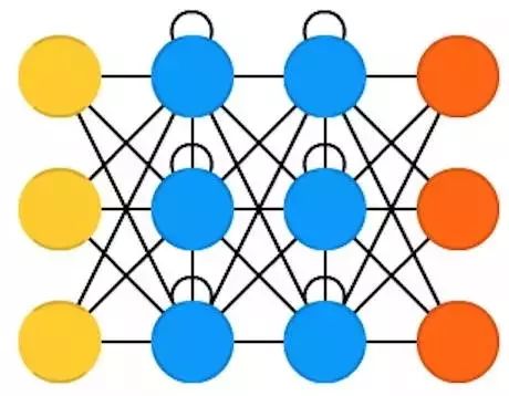
Recurrent Neural Networks (RNN) are feedforward neural networks that take time into account: they are not stateless; there is a temporal connection between channels. Neurons receive not only information from the previous layer of the neural network but also information from the previous channel. This means that the order in which you input data into the neural network and the data used to train the network is important: inputting ‘milk’, ‘cookies’ and inputting ‘cookies’, ‘milk’ will yield different results. The biggest problem with recurrent neural networks is gradient vanishing (or gradient explosion), depending on the activation function used.

In this case, information can quickly disappear over time, just as information can be lost as the depth of feedforward neural networks increases. Intuitively, this is not a big problem because they are just weights and not neuron states. However, over time, the weights have stored past information. If the weights reach 0 or 1,000,000, the previous state becomes devoid of informational value.

Convolutional neural networks can be applied to many fields; most forms of data do not have a true time axis (unlike sound or video) but can be represented in a sequential manner. For an image or a string of text, you can input one pixel or one character at each time point. Thus, time-dependent weights can be used to represent the information from the previous second rather than from several seconds ago. Generally, recurrent neural networks are a good choice for predicting future information or completing information, such as autocomplete features.

Long Short-Term Memory (LSTM) networks attempt to overcome the problems of gradient vanishing or explosion by introducing gate structures and a clearly defined memory cell. This idea is mostly inspired by circuitry rather than biology. Each neuron has a memory cell and three gate structures: input, output, and forget. The functions of these gate structures are to protect information by prohibiting or allowing the flow of information. The input gate structure determines how much information from the previous layer is stored in the current memory cell. The output gate structure performs the opposite function, determining how much information from this layer can be known to the next layer. The forget gate structure may seem strange at first, but sometimes forgetting is necessary:

If the network is learning a book and starts a new chapter, it may be necessary to forget some characters from the previous chapter.

Long Short-Term Memory networks have been shown to learn complex sequences, such as writing like Shakespeare or composing simple music. It is noteworthy that each of these gate structures assigns weights to the memory cells in the previous neuron, so generally, more resources are needed to run.

Gated Recurrent Units (GRU) are a variant of Long Short-Term Memory networks. The difference is that there are no input, output, or forget gates; it only has an update gate. This update gate determines how much information to retain from the previous state and how much information from the previous layer is retained.

This reset gate functions similarly to the forget gate in LSTM, but its position is slightly different. It always outputs the entire state but does not have an output gate. In most cases, they function very similarly to LSTM, with the biggest difference being that GRU is slightly faster and easier to run (but has less expressive power). In practice, these often cancel each other out because when you need a larger network to gain stronger expressiveness, it often offsets the performance advantage. In situations where additional expressiveness is not needed, GRU may outperform LSTM.

Neural Turing Machines (NTM) can be understood as an abstraction of LSTM, attempting to demystify (allowing us to gain insight into what is happening). Neural Turing Machines do not directly encode memory cells into neurons; their memory cells are separate. They try to combine the efficiency and permanence of conventional digital storage with the efficiency and expressiveness of neural networks. This idea is based on a content-addressable memory bank from which neural networks can read and write.

The ‘Turing’ in Neural Turing Machines comes from Turing completeness: the ability to read, write, and change states based on what it reads means it can express everything that a universal Turing machine can express.

Bidirectional Recurrent Neural Networks, Bidirectional Long Short-Term Memory Networks, and Bidirectional Gated Recurrent Units (BiRNN; BiLSTM; BiGRU) are not shown in the table because they look the same as their respective unidirectional networks. The difference is that these networks are not only connected to the past but also relate to the future.

For example, the training process of a unidirectional Long Short-Term Memory network to predict the word ‘fish’ involves inputting the word ‘fish’ letter by letter, where the recurrent connections remember the last value over time. In contrast, a bidirectional Long Short-Term Memory network inputs the next letter in the reverse channel to provide future information. This method trains the network to fill in blanks rather than predict future information; for instance, in image processing, it can fill in missing parts of an image rather than extending the boundaries of the image.

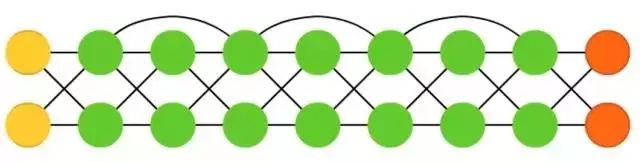
Deep Residual Networks (DRN) are feedforward neural networks with very deep architectures that have connections between neighboring layers, allowing inputs to be passed from one layer to several layers ahead (usually 2 to 5 layers). Deep Residual Networks do not map some inputs (e.g., through a 5-layer network) to outputs but learn to map some inputs to some outputs + inputs. Essentially, it adds an identity function that takes the old input as new input for the later layers.

Results show that when reaching 150 layers, these networks are very effective for pattern learning, which is much more than the conventional 2 to 5 layers. However, results have shown that these networks are essentially not built based on specific-time recurrent neural networks (RNN); they are always compared to Long Short-Term Memory networks (LSTM) without gate structures.

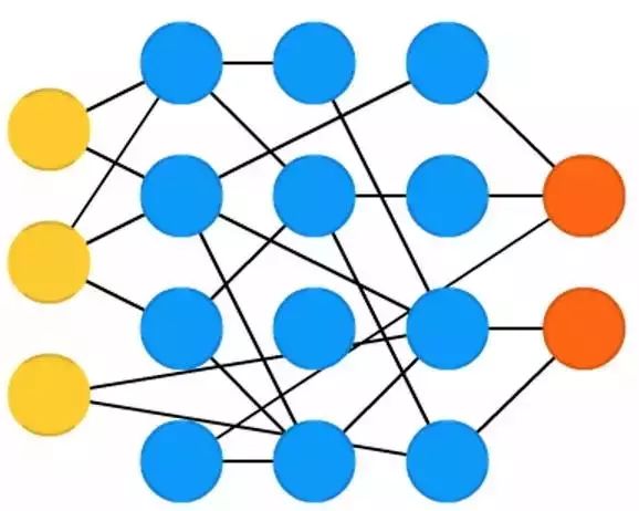
Echo State Networks (ESN) are another type of (recurrent) network. Their difference lies in the random connections between neurons (i.e., there is no unified connection pattern between layers), and their training method is also different. Unlike inputting data and then backpropagating errors, Echo State Networks first input data, feed forward, and then temporarily update the neurons. Here, the input and output layers play slightly different roles than conventional roles: the input layer is used to dominate the network, while the output layer observes the activation patterns unfolding over time. During training, only the connections between observations and hidden units are changed.

Extreme Learning Machines (ELM) are essentially feedforward neural networks with random connections. They look similar to Liquid State Machines (LSM) and Echo State Networks (ESN), but they do not have spikes or cycles. They do not use backpropagation. Instead, they randomly initialize weights and train weights through least squares fitting (minimizing the error across all functions). This gives the model slightly weaker expressiveness but is much faster than backpropagation.

Liquid State Machines (LSM) look similar to Echo State Networks (ESN). The real difference is that Liquid State Machines are a type of spiking neural network: the sigmoid activation function is replaced by a threshold function, and each neuron is a cumulative memory cell. So when updating neurons, their values are not accumulated from neighboring neurons but from their own accumulation. Once the threshold is reached, it passes its energy to other neurons. This creates a pulse-like pattern: nothing happens until it suddenly reaches the threshold.

Support Vector Machines (SVM) discover the best solutions to classification problems. Traditional SVM generally handles linearly separable data. For example, it can determine which image is Garfield and which image is Snoopy, and it cannot be any other result. During training, support vector machines can be imagined as drawing all data points (Garfield and Snoopy) on a (two-dimensional) graph and then finding how to draw a straight line to separate these data points. This line divides the data into two parts, with all Garfields on one side of the line and Snoopy on the other.

The best separating line is the one that maximizes the margin between points on either side and the line. When new data needs to be classified, we will plot this new data point on the graph and simply see which side of the line it belongs to. Using kernel tricks, they can be trained to classify n-dimensional data. This requires plotting points in a 3D graph, allowing for the separation of Snoopy, Garfield, and Simon Cat, and even more cartoon characters. Support vector machines are not always considered neural networks.

Kohonen Networks (KN; also known as Self-Organizing (Feature) Maps, SOM, SOFM) classify data using competitive learning without supervision. Data is input into the network, and then the network assesses which neuron best matches which input. The neurons are then adjusted to better match the input. During this process, neighboring neurons are moved. The extent to which neighboring neurons are moved depends on their distance to the best matching unit. Sometimes, Kohonen networks are also not considered neural networks.

This article is authorized by the Asimov Institute and translated by 36 Big Data.

To ensure the quality of publications and build a reputation, Data Express has established the“Typo Fund”, encouragingreaders to actively correct errors.

If you find any errors during your reading, please leave a message at the end of the article, or provide feedback to thebackend, and once confirmed by the editor, Data Express will reward the reporting reader with8.8 yuan red packet.

The same reader pointing out multiple errors in the same article will not change the reward. Different readers pointing out the same error will reward the first reader.

Thank you for your continued attention and support, and we hope you can supervise Data Express to produce higher quality content.