Click on the above “Beginner Learning Vision”, choose to add Star or “Top”
Essential insights delivered at the first moment
1. Concept of Convolutional Neural Networks
2. Characteristics of Convolutional Neural Networks
2.1 Local Region Connections
2.2 Weight Sharing
2.3 Downsampling
3. Structure of Convolutional Neural Networks
3.1 Convolutional Layer
3.2 Pooling Layer
4. Research Progress of Convolutional Neural Networks
1. Concept of Convolutional Neural Networks
Artificial Neural Networks (ANN) is a mathematical model of algorithms that simulates the structure and behavior of biological neural systems for distributed parallel information processing. ANN achieves information processing by adjusting the weight relationships between internal neurons. Convolutional Neural Networks (CNN), a type of feedforward neural network, consists of several convolutional layers and pooling layers, and performs exceptionally well in image processing.
In 1962, Hubel and Wiesel [1] introduced a new concept called “receptive field” through their research on the visual cortex of cats, which significantly influenced the development of artificial neural networks. The receptive field is the size of the area on the input image that corresponds to a pixel point on the feature map output by each layer of the convolutional neural network [2]. In simpler terms, a point on the feature map corresponds to a region on the input image. In 1980, Fukushima [3] proposed the neural cognitive machine and weight-sharing convolutional neural layer based on the receptive field theory from biological neuroscience, which is considered the precursor of convolutional neural networks. In 1989, LeCun [4] invented the convolutional neural network by combining the backpropagation algorithm with weight-sharing convolutional layers, and successfully applied the convolutional neural network to the handwritten character recognition system of the United States Postal Service for the first time. In 1998, LeCun [5] proposed the classic network model of convolutional neural networks, LeNet-5, which further improved the accuracy of handwritten character recognition.
The basic structure of CNN consists of an input layer, convolutional layers, pooling layers (also known as sampling layers), fully connected layers, and an output layer. Convolutional and pooling layers are generally arranged alternately, meaning a convolutional layer connects to a pooling layer, followed by another convolutional layer, and so on. Each neuron in the output feature map of a convolutional layer is locally connected to its input and computes a weighted sum with corresponding connection weights plus a bias value, resulting in the input value of that neuron. This process is equivalent to convolution, hence the name CNN [6].
2. Characteristics of Convolutional Neural Networks
Convolutional Neural Networks evolved from Multi-Layer Perceptrons (MLP) and exhibit remarkable performance in image processing due to their structural characteristics of local region connections, weight sharing, and downsampling. The uniqueness of CNN compared to other neural networks lies primarily in the aspects of weight sharing and local connections. Weight sharing makes the network structure of CNN more similar to biological neural networks. Local connections differ from traditional neural networks, where each neuron in layer n-1 connects to all neurons in layer n. Instead, neurons in layer n-1 connect only to some neurons in layer n. These two features serve to reduce the complexity of the network model and the number of weights.
2.1 Local Region Connections
In 1962, Hubel and Wiesel [1] proposed the concept of receptive fields by studying the visual hierarchical structure in biological neuroscience, where visual neurons in the cortex perceive information based on local region stimuli. The idea of local region connections is inspired by the structure of visual neurons.
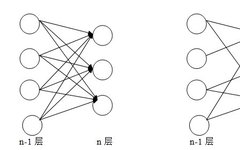
In traditional neural network structures, connections between neurons are fully connected, meaning all neurons in layer n-1 are connected to all neurons in layer n. However, in convolutional neural networks, only some neurons in layer n are connected to those in layer n-1. Figure 1 illustrates the difference between full connection and local connection, showing that in full connection, edges exist between every neuron in the previous layer and the next layer, resulting in a large number of parameters. In contrast, local connections show significantly fewer edges, greatly reducing the number of parameters.
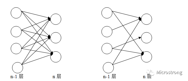
Figure 1: Comparison of Full Connection (Left) and Local Connection (Right)
2.2 Weight Sharing
In 1998, LeCun [5] released the LeNet-5 network architecture, where the term weight sharing was first introduced. Although most people now consider the AlexNet network [7] from 2012 as the beginning of deep learning, the origins of CNN can be traced back to the LeNet-5 model. Several characteristics of the LeNet-5 model were widely used in convolutional neural network research in the early 2010s, one of which is weight sharing.
In convolutional neural networks, the convolution kernels (also known as filters) in the convolutional layer act like a sliding window, moving back and forth over the entire input image with a specific stride, resulting in the feature map extracted from the input image, which represents the local features. These convolution kernels share parameters. During the training process of the entire network, the convolution kernels containing weights are updated until training is complete.
So what exactly is weight sharing?
Weight sharing means that the parameters within the same convolution kernel are shared across the entire image. For example, a 3*3*1 convolution kernel shares its 9 parameters across the entire image, without changing the weights based on different positions within the image. In simpler terms, it means using the same convolution kernel to convolve the entire image without altering its internal weight coefficients. Of course, each convolutional layer in CNN does not consist of just one convolution kernel; this explanation is for convenience.
What are the benefits of weight sharing?
Firstly, the convolution operation with weight sharing ensures that each pixel has a weight coefficient, which is shared across the entire image, significantly reducing the number of parameters in the convolution kernel and lowering the complexity of the network. Secondly, traditional neural networks and machine learning methods require complex preprocessing of images to extract features, which are then input into the neural network. The convolution operation can automatically extract features by utilizing local spatial correlations in the images.
Why does the convolutional layer have multiple convolution kernels?
Because weight sharing means that each convolution kernel can only extract one type of feature, multiple convolution kernels are needed to enhance the expressive power of CNN. However, the number of convolution kernels in each convolutional layer is a hyperparameter.
2.3 Downsampling
Downsampling is another important concept in convolutional neural networks, commonly referred to as pooling. The most common methods are max pooling, min pooling, and average pooling. The benefit of pooling is that it reduces the resolution of the image, making the entire network less prone to overfitting. Max pooling is illustrated in Figure 2.
Figure 2: Max Pooling Process
In Figure 2, the input image size is 4*4, and the maximum value is calculated in each 2*2 region. For example:  . Since the stride is 2, each 2*2 region does not overlap, resulting in an output pooling feature size of 2*2, effectively halving the resolution.
3. Structure of Convolutional Neural Networks Conclusion
In image processing, the features extracted by convolutional neural networks outperform the previous handcrafted features due to the unique organizational structure of CNN, where the interplay between convolutional and pooling layers enables CNN to extract better features from images. The network models of convolutional neural networks are diverse, but a typical CNN model generally consists of several convolutional layers, pooling layers, and fully connected layers. The role of the convolutional layer is to extract features from images; the pooling layer samples the features, allowing the use of fewer training parameters while also mitigating the overfitting of the network model. Convolutional and pooling layers typically alternate in the network, referred to as a feature extraction process, although not every convolutional layer is followed by a pooling layer. Most networks contain only three pooling layers. The final network usually consists of 1-2 fully connected layers, which connect the extracted feature maps and ultimately produce the final classification result through the classifier.
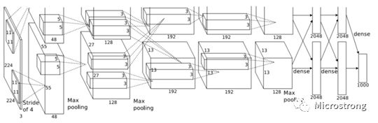
Figure 3: AlexNet Network Architecture
Figure 3 shows the convolutional neural network structure proposed by Krizhevsky et al. in 2012. This model features a dual GPU parallel structure, with half of the neurons placed in each GPU, and communication between GPUs only occurs at certain layers. The AlexNet network mainly consists of 5 convolutional layers, 3 pooling layers, and 2 fully connected layers.
3.1 Convolutional Layer
In the convolutional layer, multiple learnable convolution kernels are typically included. The feature map output from the previous layer undergoes convolution with the convolution kernels, meaning that the input items and the convolution kernels perform dot product operations, and the results are sent to an activation function to obtain the output feature map. Each output feature map may represent a combination of values from multiple input feature maps. The output value of the j-th unit in the convolutional layer l  is computed using formula (1), where
 represents the selected input feature map set, and k denotes the learnable convolution kernels. Figure 4 illustrates the specific operation process of the convolutional layer.
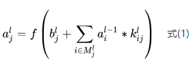
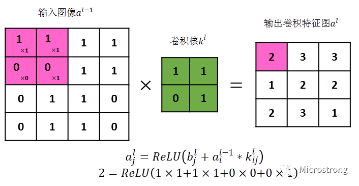
Figure 4: Illustration of Convolution Operation
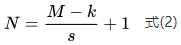
Figure 4 presents an example of a two-dimensional convolution layer, where the convolution kernel k is viewed as a sliding window that moves forward with a set stride. Here, the input image size is 4*4, M=4, the convolution kernel size is 2*2, k=2, and the stride is 1, s=1. Based on the convolution layer output calculation formula (2), the output image size N=3 can be computed.
The convolution process in Figure 4 involves convolving a 4*4 input image with a 3*3 convolution kernel, yielding a 3*3 output image. This convolution process has two drawbacks: (1) each convolution reduces the image size, and if the image is small and convolutions are performed many times, it may eventually reduce to a single pixel; (2) the edge pixels of the input image are computed only once, while the central pixels are computed multiple times, leading to a loss of edge information. To address these issues, padding (Padding) is needed for the input image.

Figure 5: Padding the Input Image
Figure 5 shows the padding of a layer of pixels around the input image matrix in Figure 4, where the padding elements are usually zeros, and the number of padded pixels is 1, P=1. Using the convolution layer output calculation formula (3), the output image size N=5 can be calculated.
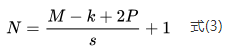
The red pixels in Figure 5 are central pixels in Figure 4, computed multiple times, while the green pixels in Figure 5 are edge pixels computed only once. It is evident that edge information is lost during the convolution process. However, with padding in Figure 5, the green pixels are no longer edge pixels and can be computed multiple times. The edge pixels of the output image, marked with a black border, are influenced by the pixel values of the input image, mitigating the loss of edge information. Additionally, according to formula (3), the output convolution feature map size becomes 5*5, solving the issue of image size reduction during convolution.
Common padding methods include Valid and Same padding:
-
Valid: No padding is used, meaning the M*M image is convolved with the k*k convolution kernel.
-
Same: Padding is applied to ensure that the output convolution feature map size equals the input image size, with the padding width P=(k-1)/2.
In computer vision, k is usually an odd number to ensure that when using Same padding, the number of padded pixels P is an integer, resulting in symmetric padding around the original image; furthermore, an odd-width convolution kernel has a center pixel that indicates the position of the convolution kernel. In my example, the convolution kernel width is 2 (an even number), so padding before convolution does not yield the same size as the original image.
3.2 Pooling Layer
The pooling layer usually follows the convolutional layer, and both alternate with each convolutional layer corresponding to a pooling layer. The activation value in pooling layer l  is computed using formula (4):

Where down(.) represents the pooling function, commonly used pooling functions include Mean-Pooling, Max-Pooling, Min-Pooling, and Stochastic-Pooling,  is the bias,
  is the multiplicative residual, and
  indicates the pooling box size used in layer l is
  . For max pooling, the maximum value of all pixels in the non-overlapping sliding box of size
  is selected from the input image. Clearly, for non-overlapping pooling, the output feature map reduces pixel-wise by
  times. The pooling layer significantly reduces the number of connections compared to the convolutional layer, thereby reducing the dimensionality of the features, which helps to avoid overfitting while providing translational invariance for the pooling output features. Figure 6 illustrates the computation processes of the three pooling methods.
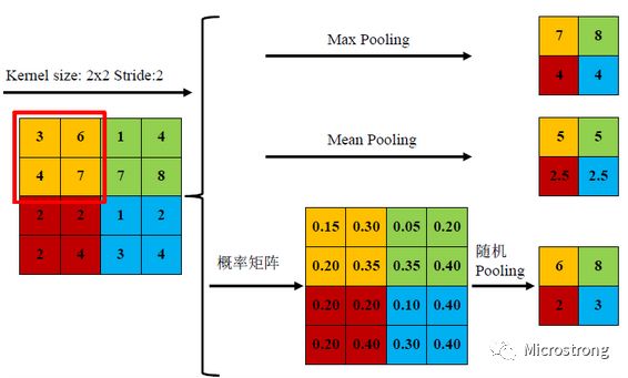
Figure 6: Computation Processes of Three Pooling Methods
The three pooling methods each have their pros and cons. Mean pooling calculates the average of all feature points, while max pooling selects the maximum value of the feature points. Stochastic pooling is intermediate, assigning probabilities based on pixel values and sub-sampling according to these probabilities. In terms of average meaning, it is similar to mean sampling, while locally, it follows the criteria of max sampling. According to Boureau’s theory [9], it can be concluded that during feature extraction, mean pooling reduces the variance of estimates caused by limited neighborhood sizes while preserving more background information; max pooling reduces the estimation mean error caused by parameter errors in the convolution layer, retaining more texture information. Stochastic pooling, while preserving information from mean pooling, introduces random probabilities that significantly affect the results and are not estimable.
4. Research Progress of Convolutional Neural Networks
As early as before 2006, a highly efficient deep learning model, CNN, was proposed. In the 1980s and 1990s, some researchers published related studies on CNN, achieving good recognition effects in several pattern recognition fields, especially in handwritten digit recognition [10][11]. However, at that time, CNN was only suitable for recognizing small images, and its performance on large-scale data was poor.
In 2012, Krizhevsky et al. [12] used an extended deep CNN to achieve the best classification results at the ImageNet Large Scale Visual Recognition Challenge (LSVRC), which drew increasing attention from researchers. AlexNet increased the network depth while adopting many new techniques: using ReLU instead of the saturated nonlinear function tanh, reducing the model’s computational complexity and significantly speeding up training; applying dropout technology to randomly set some neurons in the intermediate layers to zero during training, enhancing the model’s robustness and reducing overfitting in fully connected layers; and augmenting training samples through image translations, horizontal mirror transformations, and changes in image grayscale to reduce overfitting.
In 2014, Szegedy et al. [13] greatly increased the depth of CNN, proposing a CNN structure with over 20 layers, called GoogleNet. The GoogleNet structure employs three types of convolution operations: 1*1, 3*3, and 5*5, primarily enhancing the utilization of computer resources. Its parameters are 12 times fewer than those of AlexNet, while achieving higher accuracy, winning first place in the specified data group of image classification in LSVRC-14.
In 2014, Simonyan et al. [14] explored the importance of “depth” for CNN networks in their published article. This study demonstrated that increasing the depth of the network by continuously adding convolutional layers with 3*3 convolution kernels effectively enhances model performance when the number of weight layers reaches 16-19. The model in this study is also known as the VGG model. The VGG model replaces one convolutional layer with a larger convolution kernel with multiple convolutional layers using smaller 3*3 convolution kernels, reducing the number of parameters and making the decision function more discriminative. The VGG model achieved second place in the specified data group of image classification in the LSVRC-14 competition, confirming the significance of depth in visual representation.
Interestingly, in 2014, both GoogleNet and VGGNet participated in the LSVRC competition, achieving first and second places in classification, respectively. However, both VGG and GoogleNet have complex network structures due to their depth, leading to long training times, with VGG requiring multiple parameter fine-tunings.
In 2015, He et al. [15] utilized Residual Networks (ResNet) to address the problem of vanishing gradients. The main feature of ResNet is cross-layer connections, which introduce shortcut connections to pass inputs across layers and add them to the convolution results. ResNet contains only one pooling layer, which is connected after the last convolutional layer. ResNet enables the lower layers of the network to be sufficiently trained, with accuracy significantly improving as depth increases. The 152-layer ResNet was used in the LSVRC-15 image classification competition, achieving first place. In this literature, attempts were also made to set the depth of ResNet to 1000 and validate the model on the CIFAR-10 image processing dataset.
In recent years, the excellent characteristics of CNN, such as local connections, weight sharing, pooling operations, and multi-layer structures, have attracted considerable attention from researchers. CNN reduces the number of weights that need to be trained through weight sharing, lowers the computational complexity of the network, and enhances the generalization ability of the network through pooling operations, which provide invariance to local transformations such as translation and scaling. CNN directly inputs the raw data into the network, implicitly learning from the training data, avoiding the errors accumulated from manual feature extraction, making the entire classification process automatic. Although these characteristics have led to the widespread application of CNN in various fields, its advantages do not imply that existing networks are flawless. How to effectively train deeply hierarchical deep network models remains an area for further research. While image classification tasks can benefit from deeper convolutional networks, some methods still struggle to handle issues like occlusion or motion blur.
Discussion Group
Welcome to join the reader group of the public account to exchange ideas with peers. Currently, we have WeChat groups on SLAM, three-dimensional vision, sensors, autonomous driving, computational photography, detection, segmentation, recognition, medical imaging, GAN, algorithm competitions (which will gradually be subdivided), please scan the WeChat number below to join the group, and note: “nickname + school/company + research direction”, for example: “Zhang San + Shanghai Jiao Tong University + Vision SLAM”. Please follow the format for notes, otherwise, you will not be approved. Successfully added, you will be invited to join relevant WeChat groups based on research direction. Please do not send advertisements in the group, otherwise you will be removed from the group, thank you for your understanding.