1. Overview of KNN Algorithm

KNN can be said to be one of the simplest classification algorithms, and it is also one of the most commonly used classification algorithms. Note that KNN is a supervised learning classification algorithm, which looks somewhat similar to another machine learning algorithm, Kmeans (Kmeans is an unsupervised learning algorithm), but there is an essential difference between them. So what is the KNN algorithm? Let’s introduce it next.

2. Introduction to KNN Algorithm

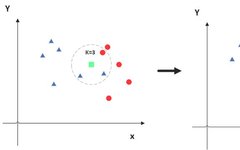
The full name of KNN is K Nearest Neighbors, meaning K nearest neighbors. From this name, we can see some clues about the KNN algorithm. The K nearest neighbors are undoubtedly crucial in determining the value of K. But what about the nearest neighbors? In fact, the principle of KNN is that when predicting a new value x, it judges which category x belongs to based on the categories of the K closest points. It sounds a bit convoluted; let’s take a look at the diagram.

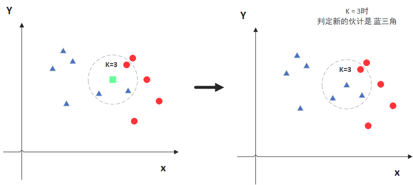
In the diagram, the green point is the one we want to predict. Assuming K=3, the KNN algorithm will find the three points closest to it (circled here) and see which category is more prevalent. For example, in this case, there are more blue triangles, so the new green point is classified as a blue triangle.

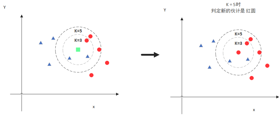
However, when K=5, the determination changes. This time, there are more red circles, so the new green point is classified as a red circle. From this example, we can see that the value of K is very important.

After understanding the general principle, let’s talk about the details, mainly two aspects: selection of K value and distance calculation.

2.1 Distance Calculation

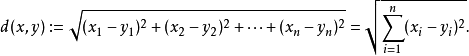
To measure the distance between points in space, there are several metrics, such as the commonly used Manhattan distance and Euclidean distance. However, in KNN, the Euclidean distance is usually used. Here is a simple introduction: for two points in a two-dimensional plane, the formula for Euclidean distance is as follows:

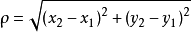
This is something you should have encountered in high school; it calculates the distance between (x1,y1) and (x2,y2). When extended to multi-dimensional space, the formula becomes:

Now we understand how to calculate the distance. The simplest and most straightforward way for KNN is to calculate the distance between the predicted point and all points, then store and sort them, selecting the top K values to see which categories are more prevalent. However, it can also be assisted by some data structures, such as a max heap; we won’t go into more detail here, but if you’re interested, you can search for knowledge about max heaps.

2.2 Choosing the K Value

From the previous diagram, we know that the choice of K is quite important. So how should we determine the value of K? The answer is through cross-validation (splitting sample data into training data and validation data in a certain ratio, such as 6:4). Start with a relatively small K value, continuously increase K, and then calculate the variance of the validation set to find a suitable K value.

After calculating the variance through cross-validation, you will generally get a graph like this: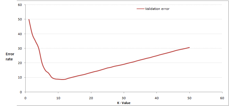

This graph is quite easy to understand. As you increase K, the error rate generally decreases at first because more surrounding samples can be referenced, improving classification performance. However, note that unlike K-means, when K increases, the error rate will be higher. This is also easy to understand; for example, if you only have 35 samples, when K increases to 30, KNN becomes almost meaningless.

So when choosing the K point, you can select a larger critical K point. When it continues to increase or decrease, the error rate will rise, such as K=10 in the graph. The specific code for determining the optimal K value will be introduced in the next section.

3. Characteristics of KNN

KNN is a non-parametric, lazy algorithm model. What does non-parametric and lazy mean?

Non-parametric means that this algorithm does not require parameters, but it implies that this model makes no assumptions about the data, in contrast to linear regression (where we always assume linear regression is a straight line). In other words, the model structure established by KNN is determined by the data, which is more in line with reality, as real situations often do not match theoretical assumptions.

Lazy also has a specific meaning. Think about it: as a classification algorithm, logistic regression requires a lot of training (training) on the data before obtaining an algorithm model. However, the KNN algorithm does not require this; it does not have a clear training data process, or rather, this process is very quick.

Advantages and Disadvantages of KNN Algorithm

Understanding the advantages and disadvantages of the KNN algorithm can help us make more informed decisions when choosing a learning algorithm. So let’s take a look at the advantages and defects of the KNN algorithm!

Advantages of KNN Algorithm

1. Simple and easy to use; compared to other algorithms, KNN is relatively straightforward. Even without a high level of mathematical foundation, one can understand its principles.

2. Fast model training time; as mentioned above, the KNN algorithm is lazy, so we won’t elaborate further.

3. Good prediction performance.

4. Not sensitive to outliers.

Disadvantages of KNN Algorithm

1. High memory requirements because the algorithm stores all training data.

2. Prediction phase may be slow.

3. Sensitive to irrelevant features and data scale.

As for when to choose to use the KNN algorithm, this chart from sklearn gives us an answer. 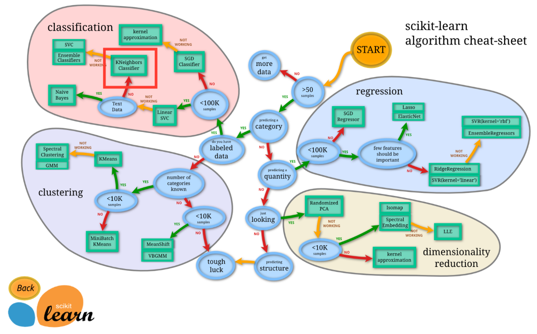In simple terms, when you need to use a classification algorithm and the data is relatively large, you can try using the KNN algorithm for classification.

Okay, this concludes the introduction to the KNN algorithm. The next section will analyze the parameters of sklearn and the selection of K values.