Translator | Zhu Xianzhong
This article will comprehensively explain what Generative Adversarial Networks (GANs) are, how they work, and how to build such a network in a Python environment.
Recently, the data science community has been vigorously promoting Generative Adversarial Networks (GANs). However, as you begin to understand them, you will immediately grasp the reason behind it. The GAN architecture is simply a genius design, primarily because it “unleashes” the tremendous potential for generating and augmenting real data.
In this article, I will first introduce you to the basics of GANs and show you how to write a GAN in a Python environment using the Keras/TensorFlow library. In summary, it mainly includes the following:
-
GAN in Machine Learning Algorithms
-
An Intuitive Explanation of GAN Architecture and Its Working Mechanism
-
A Detailed Python Example Demonstrating How to Build a GAN from Scratch
GAN in Machine Learning Algorithms
Even experienced data scientists can easily get lost among hundreds of different machine learning algorithms. To summarize these algorithms, I categorized some of the most common ones and created a visual sunburst chart.
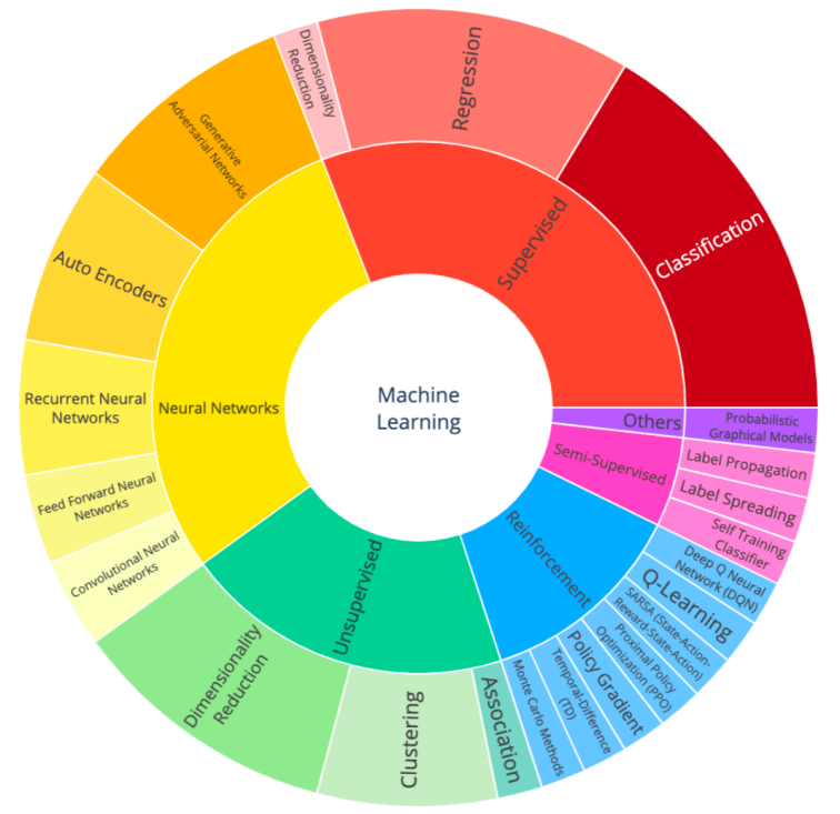
Sunburst Chart of Machine Learning Algorithm Classification
Note that some of these algorithms are quite flexible and can be applied to different tasks. Therefore, no classification algorithm will ever be the perfect classification algorithm. Nevertheless, being able to see such a high-level view is still of significant importance.
Note: The chart presented in the original text is interactive; by clicking on different category links, you can learn more corresponding tip information. Therefore, the static chart provided in this translation can only leave you with some regret.
You will find that GAN is just a subclass of neural networks, which further includes several different subtypes, such as basic GANs (the focus of this article), conditional GANs (cGANs), deep convolutional GANs (DCGANs), and other types that I will introduce in future articles.
Intuitive Explanation of GAN Architecture and Its Working Mechanism
Generative Adversarial Networks are deep learning machines that combine two separate models into one architecture. These two components are:
These two models compete against each other in a zero-sum game. The generator model attempts to generate new data samples that are similar to the data samples in the problem domain. Meanwhile, the discriminator tries to identify whether the given samples are fake (from the generator) or real (from the actual data domain).
The competition between the generator and the discriminator makes them adversaries, hence the name GAN.
First, let’s analyze the generator model and see how it generates new data samples.
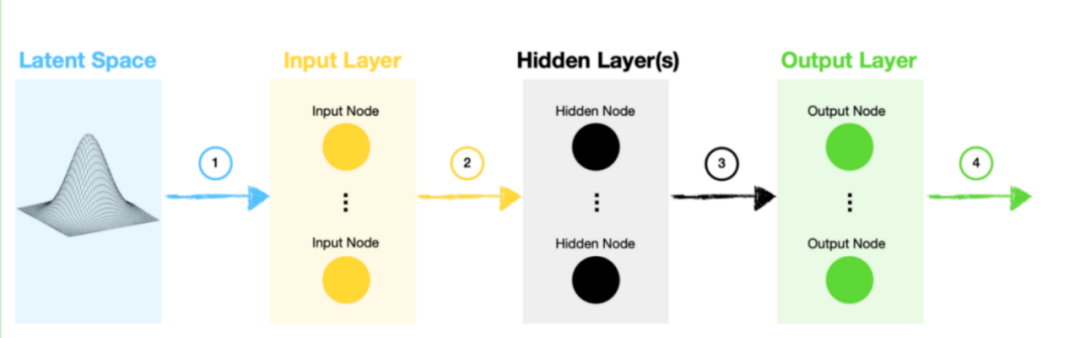
1. The generator model samples a random vector from the latent space. This space follows a Gaussian distribution, and the dimensions are specified by us. Since we use the random vector as the input to the neural network, the random vector becomes the seed data for this generation process.
2. The input follows the standard path of a network with one or more hidden layers. In the case of a simple GAN architecture, this will be a set of tightly connected layers, while a deep convolutional GAN (DCGAN) also includes convolutional layers.
3. Data flows into the output layer, where we can make final adjustments to ensure that the generator’s output data contains the desired shape to feed into the discriminator.
4. Finally, we can use these fake (generated) samples to test and “fool” the discriminator.
Next, let’s see how to construct the discriminator model.
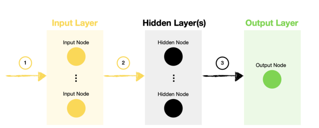
Discriminator Model
1. The input to the discriminator model is a combination of real samples (extracted from the problem domain) and fake samples (created by the generator model).
2. Data flows through a network with one or more hidden layers, just like data in any other neural network.
3. Once we reach the output layer, the discriminator can decide whether the sample is real or fake (generated).
In summary, the discriminator is no different from a standard neural network classification model.
Generative Adversarial Networks combine the competing generator and discriminator models. The following GAN architecture diagram illustrates how the two models are interconnected.
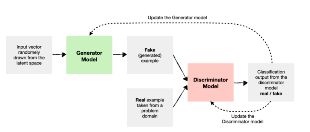
GAN Model Architecture Diagram
As shown in the figure, we input fake (generated) and real sample data into the discriminator model to train it to distinguish between the two types.
As the discriminator becomes better at distinguishing real and fake sample data, the weights and biases of the generator model are updated to produce more convincing fake sample data.
This process will be repeated several times (according to the specified number of generations) until both the generator and discriminator become better at their respective tasks. Ultimately, in extreme cases, the output of the generator model becomes indistinguishable from the actual output, and the discriminator model converges to a neutral prediction result of about 0.5.
Building a GAN Example Based on Python from Scratch
The purpose of this example is to fundamentally understand how GANs work. Therefore, we will apply it to a simple problem.
Preparation
We will use the following libraries:
-
Pandas, Numpy, and Math libraries for data generation and manipulation
-
Matplotlib, Graphviz, and Plotly (optional) for data visualization
-
TensorFlow/Keras for building neural networks
First, let’s import the libraries:
# TensorFlow / Keras
from tensorflow import keras # for building neural networks
print('TensorFlow/Keras: %s' % keras.__version__) # print version
from keras.models import Sequential # for assembling neural network models
from keras.layers import Dense # add some layers to the neural network model
from tensorflow.keras.utils import plot_model # plot model diagram
# Data manipulation
import numpy as np # for data manipulation
print('numpy: %s' % np.__version__) # print version
import pandas as pd # for data manipulation
print('pandas: %s' % pd.__version__) # print version
import math # for generating real data (in this case, a circle)
# Visualization
import matplotlib
import matplotlib.pyplot as plt # for data visualization
print('matplotlib: %s' % matplotlib.__version__) # print version
import graphviz # for showing model diagram
print('graphviz: %s' % graphviz.__version__) # print version
import plotly
import plotly.express as px # for data visualization
print('plotly: %s' % plotly.__version__) # print version
# Other tools
import sys
import os
# Assign the main directory to a variable
main_dir=os.path.dirname(sys.path[0])
Swipe left to view the complete code
The above code will print the version information of the packages used in this example, as follows:
TensorFlow/Keras: 2.7.0 numpy: 1.21.4 pandas: 1.3.4 matplotlib: 3.5.1 graphviz: 0.19.1 plotly: 5.4.0
Next, we will create a circle and obtain the coordinates of points on its edge (circumference). Then, we will train the generator and discriminator to let GAN “recognize” and “generate” such a circle.
# Function to get coordinates of points on the edge (circumference)
def PointsInCircum(r,n=100):
    return [(math.cos(2*math.pi/n*x)*r,math.sin(2*math.pi/n*x)*r) for x in range(0,n+1)]
# Save a set of real number coordinates of a circle with a radius of 2
circle=np.array(PointsInCircum(r=2,n=1000))
# Plot the chart
plt.figure(figsize=(15,15), dpi=400)
plt.title(label='Real circle to be learned by the GAN generator', loc='center')
plt.scatter(circle[:,0], circle[:,1], s=5, color='black')
plt.show()
Swipe left to view the complete code
The above code will generate 1000 points and plot a circle.
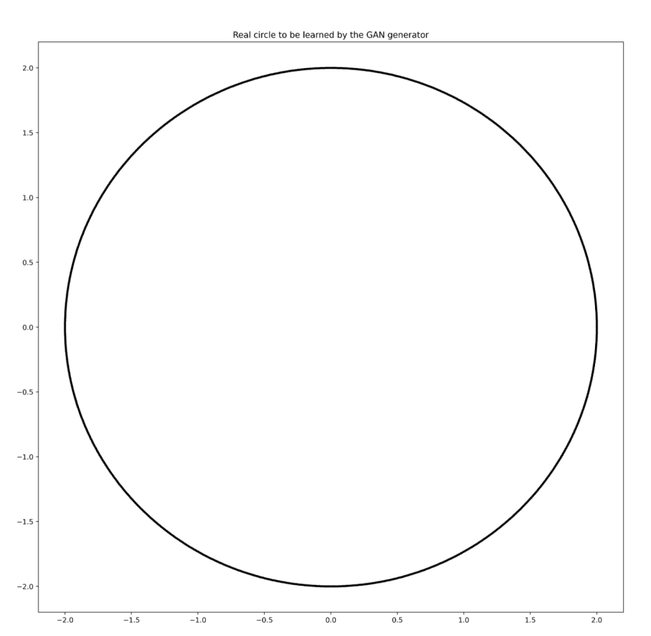
Circle composed of 1000 points
Creating the GAN Model
Now that we have prepared the data, let’s start defining and assembling our model. We will start with the generator:
# Define the generator model
def generator(latent_dim, n_outputs=2):
    model = Sequential(name="Generator") # Model
    # Add layers
    model.add(Dense(32, activation='relu', kernel_initializer='he_uniform', input_dim=latent_dim, name='Generator-Hidden-Layer-1')) # Hidden layer
    model.add(Dense(16, activation='relu', kernel_initializer='he_uniform', name='Generator-Hidden-Layer-2')) # Hidden layer
    model.add(Dense(n_outputs, activation='linear', name='Generator-Output-Layer')) # Output layer
    return model
# Instantiate
gen_model = generator(latent_dim)
# Display model summary information and plot model diagram
gen_model.summary()
plot_model(gen_model, show_shapes=True, show_layer_names=True, dpi=400)
Swipe left to view the complete code
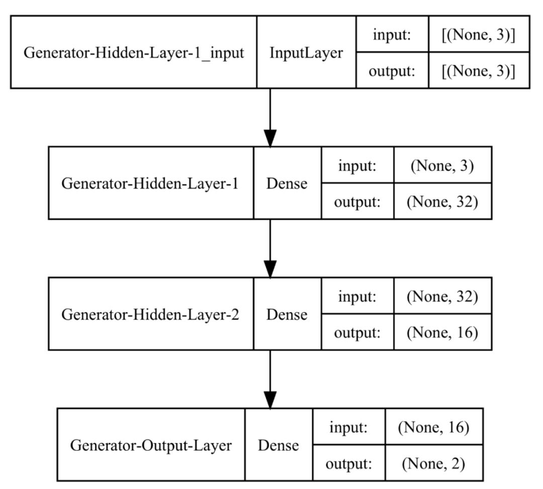
As you can see, our generator has three input nodes because we decided to draw a random vector from a three-dimensional latent space. Note that we can freely choose the dimension of the latent space.
At the same time, the output result shows two values corresponding to the x and y coordinates of a point in two-dimensional space.
Next, we will build the discriminator model:
# Build the discriminator model
def discriminator(n_inputs=2):
    model = Sequential(name="Discriminator") # Model
    # Add layers
    model.add(Dense(32, activation='relu', kernel_initializer='he_uniform', input_dim=n_inputs, name='Discriminator-Hidden-Layer-1')) # Hidden layer
    model.add(Dense(16, activation='relu', kernel_initializer='he_uniform', name='Discriminator-Hidden-Layer-2')) # Hidden layer
    model.add(Dense(1, activation='sigmoid', name='Discriminator-Output-Layer')) # Output layer
    # Compile model
    model.compile(loss='binary_crossentropy', optimizer='adam', metrics=['accuracy'])
    return model
# Instantiate
dis_model = discriminator()
# Display model summary information and plot model diagram
dis_model.summary()
plot_model(dis_model, show_shapes=True, show_layer_names=True, dpi=400)
Swipe left to view the complete code
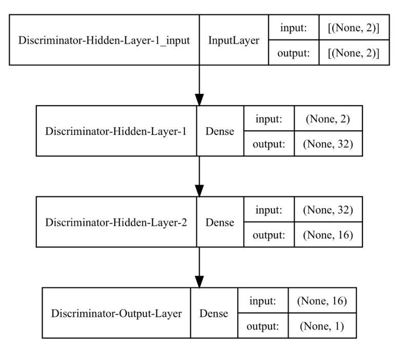
Discriminator Model Diagram
The discriminator input takes two values, aligned with the generator output. At the same time, the discriminator output is just one value, indicating how confident the model is about the data being real/fake.
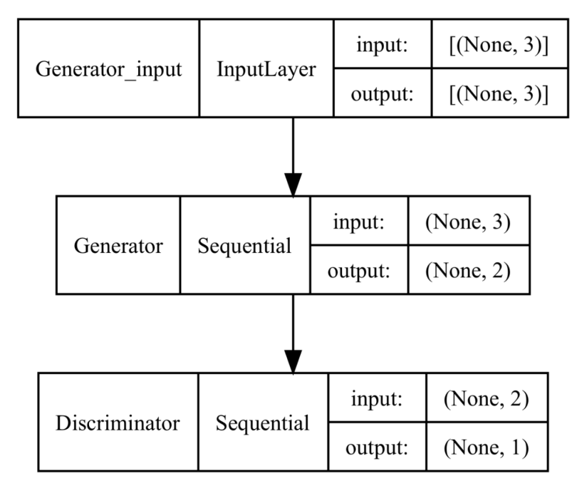
Next, we combine these two models to create the GAN. One key detail in the code below is that we make the discriminator model untrainable. We do this because we want to train the discriminator separately using real and fake (generated) data. Later, you will see how we achieve this.
def def_gan(generator, discriminator):
    # We do not want to train the discriminator's weights at this stage. So make it untrainable
    discriminator.trainable = False
    # Combine the two models
    model = Sequential(name="GAN") # GAN Model
    model.add(generator) # Add generator
    model.add(discriminator) # Add discriminator
    # Compile model
    model.compile(loss='binary_crossentropy', optimizer='adam')
    return model
# Instantiate
 gan_model = def_gan(gen_model, dis_model)
# Display model summary information and plot model diagram
 gan_model.summary()
plot_model(gan_model, show_shapes=True, show_layer_names=True, dpi=400)
Swipe left to view the complete code
Preparing Inputs for the Generator and Discriminator
We will create three simple functions to assist us in sampling and generating data for both models.
The first function is responsible for sampling real point data from the circle;
The second function is responsible for extracting random vectors from the latent space;
The third function is responsible for passing the latent variables to the generator model to generate pseudo sample data.
# Construct functions to sample random point data from our circle
def real_samples(n):
    # Real sample data
    X = circle[np.random.choice(circle.shape[0], n, replace=True), :]
    # Class labels
    y = np.ones((n, 1))
    return X, y
# Generate point data on the latent space; we will use this for the generator's input data later
def latent_points(latent_dim, n):
    # Generate point data on the latent space
    latent_input = np.random.randn(latent_dim * n)
    # Reshape: make it the batch output for the network
    latent_input = latent_input.reshape(n, latent_dim)
    return latent_input
# Generate n pseudo sample data using the generator, combined with class label information
def fake_samples(generator, latent_dim, n):
    # Generate points in the latent space
    latent_output = latent_points(latent_dim, n)
    # Predict output (e.g., generate pseudo sample data)
    X = generator.predict(latent_output)
    # Create class labels
    y = np.zeros((n, 1))
    return X, y
Swipe left to view the complete code
Model Training and Evaluation
The last two functions will help us train the model and evaluate the resulting data at specified intervals.
First, let’s create a function to evaluate model performance:
def performance_summary(epoch, generator, discriminator, latent_dim, n=100):
    # Get samples of real data
    x_real, y_real = real_samples(n)
    # Evaluate the discriminator on real data
    _, real_accuracy = discriminator.evaluate(x_real, y_real, verbose=1)
    # Get fake (generated) samples
    x_fake, y_fake = fake_samples(generator, latent_dim, n)
    # Evaluate the discriminator on fake (generated) data
    _, fake_accuracy = discriminator.evaluate(x_fake, y_fake, verbose=1)
    # Summarize discriminator performance
    print("Epoch number: ", epoch)
    print("Discriminator Accuracy on REAL points: ", real_accuracy)
    print("Discriminator Accuracy on FAKE (generated) points: ", fake_accuracy)
    # Create a 2D scatter plot to show real and fake (generated) data points
    plt.figure(figsize=(4,4), dpi=150)
    plt.scatter(x_real[:, 0], x_real[:, 1], s=5, color='black')
    plt.scatter(x_fake[:, 0], x_fake[:, 1], s=5, color='red')
    plt.show()
Swipe left to view the complete code
As you can see, the above function evaluates the discriminator on real and fake (generated) points separately. Then it plots a 2D scatter plot to show the positions of these points in two-dimensional space.
Finally, the training function is as follows:
def train(g_model, d_model, gan_model, latent_dim, n_epochs=10001, n_batch=256, n_eval=1000):
    # The batches we train the discriminator will include half real points and half fake (generated) points
    half_batch = int(n_batch / 2)
    # We manually enumerate generations (epochs)
    for i in range(n_epochs):
        # Train the discriminator
        # Prepare real sample data
        x_real, y_real = real_samples(half_batch)
        # Prepare fake (generated) sample data
        x_fake, y_fake = fake_samples(g_model, latent_dim, half_batch)
        # Train the discriminator using both real and fake samples
        d_model.train_on_batch(x_real, y_real)
        d_model.train_on_batch(x_fake, y_fake)
        # Generator training
        # Get points from the latent space to use as input for the generator
        x_gan = latent_points(latent_dim, n_batch)
        # When we generate fake samples, we want the GAN generator model to create samples similar to the real ones
        # Therefore, we want to pass the labels corresponding to the real samples, i.e., y=1 instead of 0.
        y_gan = np.ones((n_batch, 1))
        # Train the generator via a composite GAN model
        gan_model.train_on_batch(x_gan, y_gan)
        # Evaluate the model at every n_eval epochs
        if (i) % n_eval == 0:
            performance_summary(i, g_model, d_model, latent_dim)
Swipe left to view the complete code
As mentioned earlier, we train the discriminator separately by passing a batch of 50% real and 50% fake (generated) sample data. Meanwhile, the generator training is done through the combined GAN model.
Experimental Results
Let’s call the training function to display some results from the above experiments:
# Train the GAN model
train(gen_model, dis_model, gan_model, latent_dim)
Swipe left to view the complete code
The following images show the results output at epoch 0:
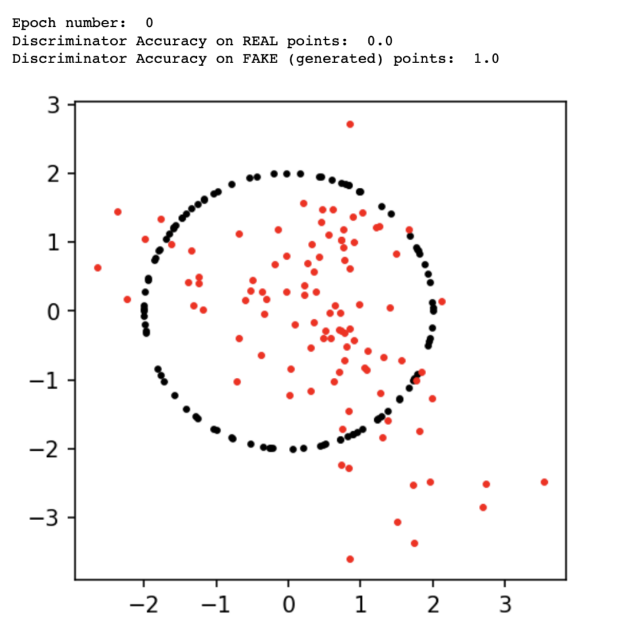
GAN Performance After Epoch 0
The results output at epoch 3,000:
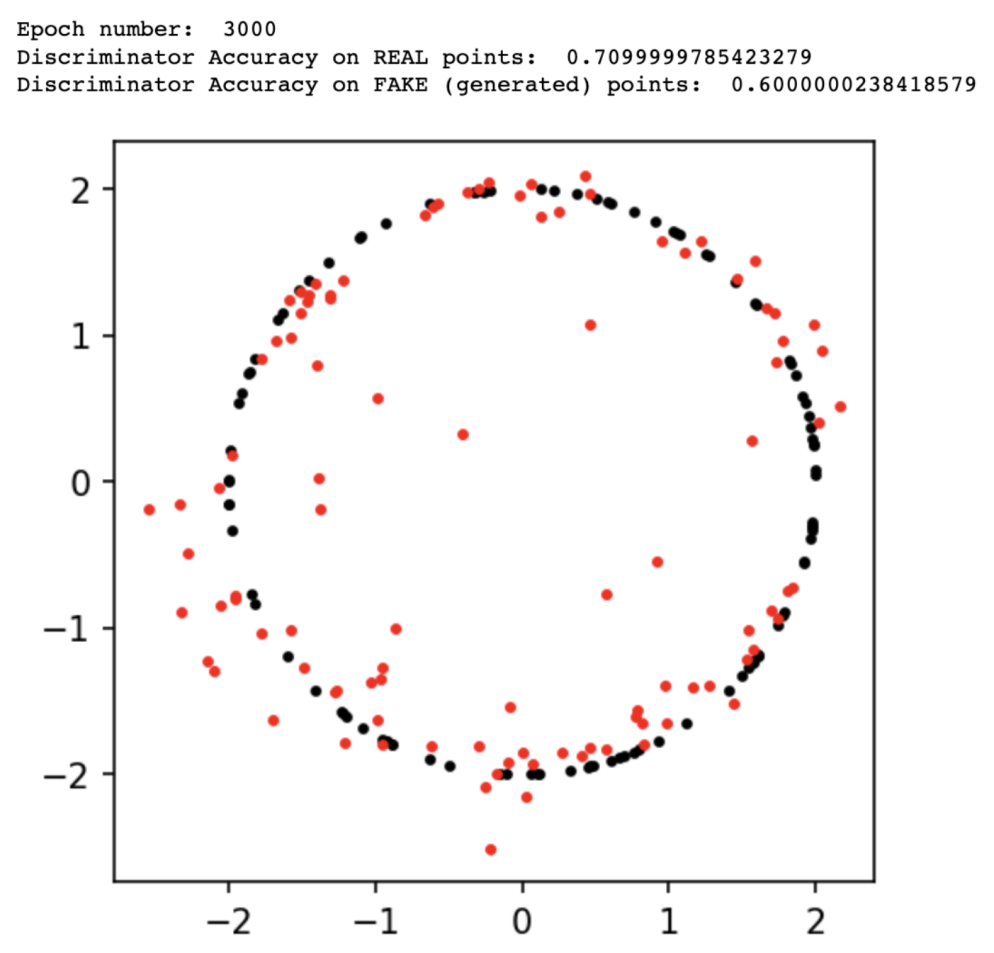
GAN Performance After Epoch 3,000
The results output at epoch 10,000:
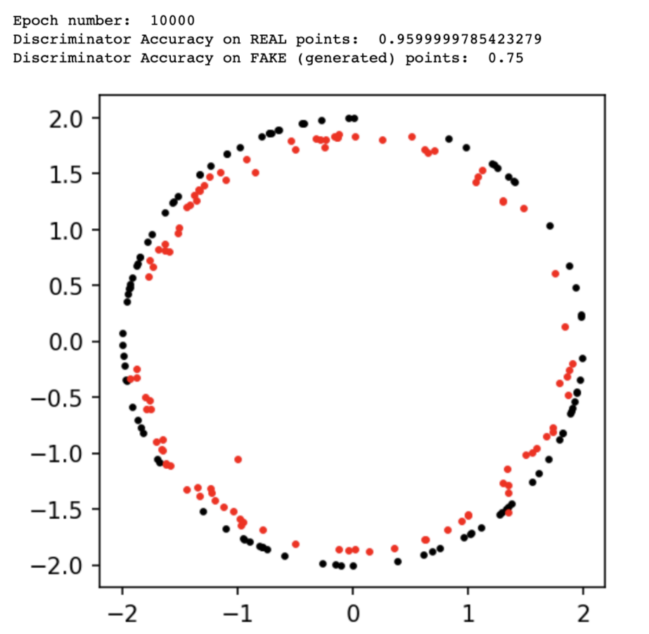
GAN Performance After Epoch 10,000
We can see that the generator improved at each step. However, after 10,000 epochs, the discriminator still performed well, able to recognize most real samples and most fake (generated) samples. Therefore, we can continue training the model for the next 10,000 epochs for better results.
Another way to compare the performance of the above models is to look at the summary statistics of the distributions of real and fake points:
# Generate 1000 pseudo sample data
x_fake, y_fake = fake_samples(gen_model, latent_dim, 1000)
df_fake = pd.DataFrame(x_fake, columns=['x dimension', 'y dimension'])
# 1000 real sample data points
x_real, y_real = real_samples(1000)
df_real = pd.DataFrame(x_real, columns=['x dimension', 'y dimension'])
# Display summary statistics
print("Distribution statistics of fake (generated) points")
print(df_fake.describe())
print("----------------------------------------")
print("Distribution statistics of real points")
print(df_real.describe())
Swipe left to view the complete code
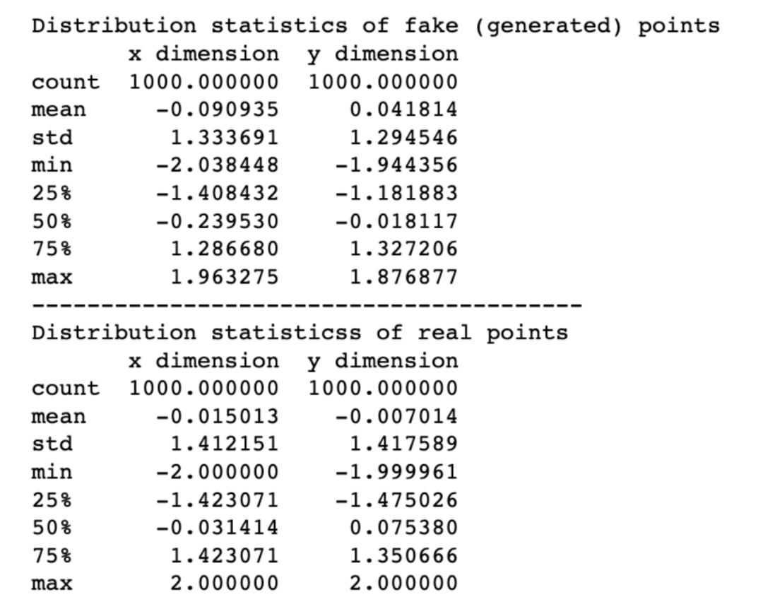
Comparison of Distribution Statistics of Real and Fake (Generated) Points
The experimental data above clearly indicates that the distribution differences are relatively small.
I hope that after reading this article, you will have a good understanding of how GAN networks work.
About the Translator
Zhu Xianzhong, editor of the 51CTO community, expert blogger and lecturer at 51CTO, a computer teacher at a university in Weifang, and a veteran in the programming world. Early on, he focused on various Microsoft technologies (co-authored three technical books related to ASP.NET AJX and Cocos 2d-X). In the past decade, he has immersed himself in the open-source world (familiar with popular full-stack web development technologies), and understands IoT development technologies based on OneNet/AliOS+Arduino/ESP32/Raspberry Pi, as well as big data development technologies like Scala+Hadoop+Spark+Flink.
https://towardsdatascience.com/gans-generative-adversarial-networks-an-advanced-solution-for-data-generation-2ac9756a8a99