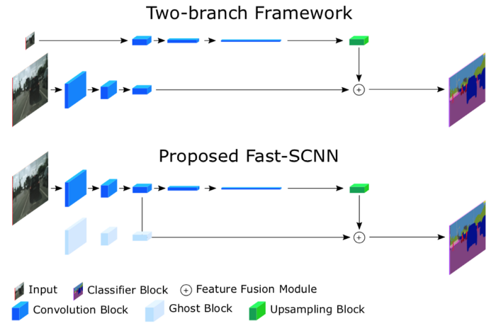
Fast Segmentation Convolutional Neural Network (Fast-SCNN) is a real-time semantic segmentation model designed for high-resolution image data, suitable for efficient computation on low-memory embedded devices. The original paper was authored by: Rudra PK Poudel, Stephan Liwicki, and Roberto Cipolla. The code used in this article is not the official implementation by the authors but an attempt to reconstruct the model described in the paper.

With the rise of autonomous vehicles, there is an urgent need for a model that can process inputs in real-time. Although there are some state-of-the-art offline semantic segmentation models available, they tend to be large in size, memory-intensive, and computationally heavy, which Fast-SCNN aims to address.

Some key aspects of Fast-SCNN include:

1. Real-time segmentation on high-resolution images (1024 x 2048px)
2. Achieves an average IOU of 68% accuracy
3. Processes 123.5 frames per second on the Cityscapes dataset
4. Requires no extensive pre-training
5. Combines high-resolution spatial details with low-resolution extracted deep features

Furthermore, Fast-SCNN utilizes state-of-the-art models from popular techniques to ensure the aforementioned performance, such as the Pyramid Pooling Module (PPM) used in PSPNet, the inverted residual bottleneck layer used in MobileNet V2, as well as the feature fusion module in ContextNet. It also leverages deep features extracted from low-resolution data and spatial details extracted from high-resolution data to ensure better and faster segmentation.

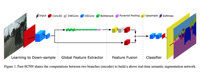
Now let’s begin the exploration and implementation of Fast-SCNN. Fast-SCNN consists of four main components. They are:

1. Learning Downsampling
2. Global Feature Extractor
3. Feature Fusion
4. Classifier

1. Learning Downsampling

So far, we know that the first few layers of deep convolutional neural networks extract low-level features from images such as edges and corners. Therefore, to fully utilize these features and make them available for further layers, learning downsampling is required. It serves as a rough global feature extractor that can be reused and shared by other modules in the network.

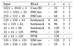
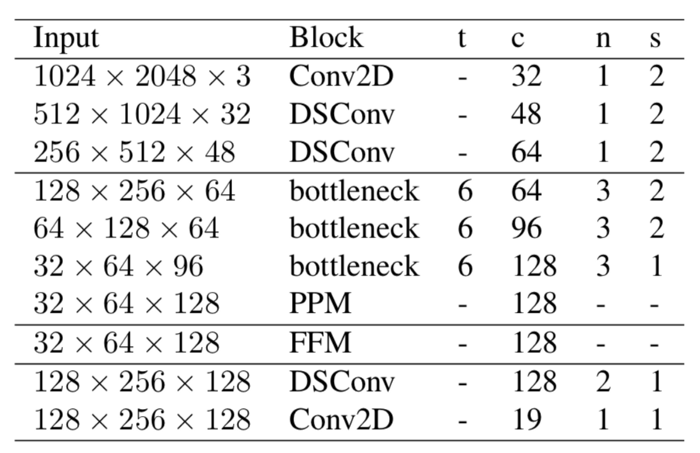
The learning downsampling module uses three layers to extract these global features. They are: a Conv2D layer followed by two depthwise separable convolution layers. In the implementation, a Batchnorm layer and ReLU activation are used after each Conv2D and depthwise separable Conv layer, as it is a standard practice to introduce Batchnorm and activation after these layers. Here, all three layers use a stride of 2 and a kernel size of 3×3.

Now, let’s first implement this module. First, we install TensorFlow 2.0. We can simply use Google Colab to start our implementation. You can easily install it using the following command:

!pip install tensorflow-gpu==2.0.0

Here, ‘-gpu’ indicates that my Google Colab notebook is using a GPU, and in your case, if you do not want to use it, you can simply remove ‘-gpu’, and then the TensorFlow installation will utilize the system’s CPU.

Then import TensorFlow:

import tensorflow as tf

Now, let’s first create the input layer for our model. In TensorFlow 2.0, using the TF.Keras high-level API, we can do this:

input_layer = tf.keras.layers.Input(shape=(2048, 1024, 3), name = 'input_layer')

This input layer is the entry point of the model we are going to build. Here we are using the function API of Tf.Keras. The reason for using the function API instead of the sequential API is that it provides the flexibility needed to build this specific model.

Next, let’s define the layers of the learning downsampling module. To simplify and reuse the process, I created a custom function that checks whether the layer I want to add is a Conv2D layer or a depthwise separable layer, and then checks if I want to add ReLU at the end of the layer. Using this code block makes the implementation of convolution easy to understand and reuse throughout the process.

def conv_block(inputs, conv_type, kernel, kernel_size, strides, padding='same', relu=True):
  
  if(conv_type == 'ds'):
    x = tf.keras.layers.SeparableConv2D(kernel, kernel_size, padding=padding, strides = strides)(inputs)
  else:
    x = tf.keras.layers.Conv2D(kernel, kernel_size, padding=padding, strides = strides)(inputs)  
  
  x = tf.keras.layers.BatchNormalization()(x)
  
  if (relu):
    x = tf.keras.activations.relu(x)
  
  return x

In TF.Keras, the Convolutional layer is defined as tf.keras.layers, and the depthwise separable layer is tf.keras.layers.SeparableConv2D.

Now, let’s add layers to the module by calling the custom function with appropriate parameters:

lds_layer = conv_block(input_layer, 'conv', 32, (3, 3), strides = (2, 2))
lds_layer = conv_block(lds_layer, 'ds', 48, (3, 3), strides = (2, 2))
lds_layer = conv_block(lds_layer, 'ds', 64, (3, 3), strides = (2, 2))

2. Global Feature Extractor

The purpose of this module is to capture global context for segmentation. It directly takes the output from the learning downsampling module. In this section, we introduce different bottleneck residual blocks and a special module, the Pyramid Pooling Module (PPM), to aggregate different region-based contextual information.

Let’s start with the bottleneck residual block.

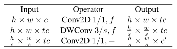
The above is the description of the bottleneck residual block in this article. Similar to above, let’s use the tf.keras high-level API to implement.

We first customize some functions based on the description in the table above. We start with the residual block, which will call our custom conv_block function to add Conv2D, then add DepthWise Conv2D layers, followed by the point-wise convolution layer, as described in the table above. Finally, we add the output of the point-wise convolution to the original input to make it a residual.

def _res_bottleneck(inputs, filters, kernel, t, s, r=False):
    
    tchannel = tf.keras.backend.int_shape(inputs)[-1] * t

    x = conv_block(inputs, 'conv', tchannel, (1, 1), strides=(1, 1))

    x = tf.keras.layers.DepthwiseConv2D(kernel, strides=(s, s), depth_multiplier=1, padding='same')(x)
    x = tf.keras.layers.BatchNormalization()(x)
    x = tf.keras.activations.relu(x)

    x = conv_block(x, 'conv', filters, (1, 1), strides=(1, 1), padding='same', relu=False)

    if r:
        x = tf.keras.layers.add([x, inputs])
    return x

This bottleneck residual block is added multiple times in the architecture, and the number of additions is indicated by the ‘n’ parameter in the table. Therefore, to add ‘n’ times as described in this article, we introduce another custom function to accomplish this task.

def bottleneck_block(inputs, filters, kernel, t, strides, n):
  x = _res_bottleneck(inputs, filters, kernel, t, strides)
  
  for i in range(1, n):
    x = _res_bottleneck(x, filters, kernel, t, 1, True)

  return x

gfe_layer = bottleneck_block(lds_layer, 64, (3, 3), t=6, strides=2, n=3)
gfe_layer = bottleneck_block(gfe_layer, 96, (3, 3), t=6, strides=2, n=3)
gfe_layer = bottleneck_block(gfe_layer, 128, (3, 3), t=6, strides=1, n=3)

Here, you will notice that the first input of these bottleneck blocks comes from the output of the learning downsampling module. The last block of this global feature extractor part is the Pyramid Pooling Module, abbreviated as PPM.

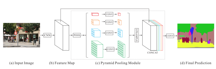
PPM uses the feature map output from the previous convolution layer, then applies multiple sub-region average pooling and upsampling functions to obtain feature representations from different sub-regions, which are then concatenated together, thus embedding local and global contextual information, making the image segmentation process more accurate.

Using TF.Keras to implement, we use another custom function:

def pyramid_pooling_block(input_tensor, bin_sizes):
  concat_list = [input_tensor]
  w = 64
  h = 32

  for bin_size in bin_sizes:
    x = tf.keras.layers.AveragePooling2D(pool_size=(w//bin_size, h//bin_size), strides=(w//bin_size, h//bin_size))(input_tensor)
    x = tf.keras.layers.Conv2D(128, 3, 2, padding='same')(x)
    x = tf.keras.layers.Lambda(lambda x: tf.image.resize(x, (w,h)))(x)

    concat_list.append(x)

  return tf.keras.layers.concatenate(concat_list)

We add this PPM module, which will take input from the last bottleneck block.

gfe_layer = pyramid_pooling_block(gfe_layer, [2,4,6,8])

Here, the second parameter is the number of bins to be provided to the PPM module, which is the same as the number of bins used in the paper. These bins are used for AveragePooling in different sub-regions, as described in the custom function above.

3. Feature Fusion

In this module, two inputs are added together to better represent the segmentation. The first is the high-level features extracted from the learning downsampling module, which first undergoes point-wise convolution before being added to the second input. No activation is applied at the end of the point-wise convolution here.

ff_layer1 = conv_block(lds_layer, 'conv', 128, (1,1), padding='same', strides= (1,1), relu=False)

The second input is the output of the global feature extractor. But before adding the second input, it first undergoes upsampling (4,4), followed by DepthWise convolution, and finally another point-wise convolution. No activation is added in the output of the point-wise convolution; activation is introduced after the two inputs are added together.

This is the low-resolution operation implemented using TF.Keras:

ff_layer2 = tf.keras.layers.UpSampling2D((4, 4))(gfe_layer)
ff_layer2 = tf.keras.layers.DepthwiseConv2D(128, strides=(1, 1), depth_multiplier=1, padding='same')(ff_layer2)
ff_layer2 = tf.keras.layers.BatchNormalization()(ff_layer2)
ff_layer2 = tf.keras.activations.relu(ff_layer2)
ff_layer2 = tf.keras.layers.Conv2D(128, 1, 1, padding='same', activation=None)(ff_layer2)

Now, let’s add these two inputs to the feature fusion module.

ff_final = tf.keras.layers.add([ff_layer1, ff_layer2])
ff_final = tf.keras.layers.BatchNormalization()(ff_final)
ff_final = tf.keras.activations.relu(ff_final)

4. Classifier

In the classifier part, two depthwise separable convolution layers and one point-wise convolution layer are introduced. BatchNorm layers and ReLU activation are also performed after each layer.

It is worth noting that in the original paper, there is no mention of adding upsampling and Dropout layers after the point-wise convolution layer, but in the later part of this article, it is described that these layers are added after the point-wise convolution layer. Therefore, in the implementation, I also introduced these two layers as per the paper’s requirements.

After performing upsampling according to the final output requirements, SoftMax will serve as the activation of the last layer.

classifier = tf.keras.layers.SeparableConv2D(128, (3, 3), padding='same', strides = (1, 1), name = 'DSConv1_classifier')(ff_final)
classifier = tf.keras.layers.BatchNormalization()(classifier)
classifier = tf.keras.activations.relu(classifier)

classifier = tf.keras.layers.SeparableConv2D(128, (3, 3), padding='same', strides = (1, 1), name = 'DSConv2_classifier')(classifier)
classifier = tf.keras.layers.BatchNormalization()(classifier)
classifier = tf.keras.activations.relu(classifier)

classifier = conv_block(classifier, 'conv', 19, (1, 1), strides=(1, 1), padding='same', relu=True)

classifier = tf.keras.layers.Dropout(0.3)(classifier)

classifier = tf.keras.layers.UpSampling2D((8, 8))(classifier)
classifier = tf.keras.activations.softmax(classifier)

Compile the Model

Now that we have added all the layers, let’s create the final model and compile it. To create the model, we use the function API from TF.Keras as described above. Here, the input of the model is the initial input layer described in the learning downsampling module, and the output is the output of the final classifier.

fast_scnn = tf.keras.Model(inputs = input_layer , outputs = classifier, name = 'Fast_SCNN')

Now, let’s compile it with an optimizer and a loss function. In the original paper, the authors used an SGD optimizer with a momentum value of 0.9 and a batch size of 12 during training. They also used a polynomial learning rate strategy with a base value of 0.045 and a power of 0.9. For simplicity, I have not used any learning rate strategy here, but if needed, you can add it yourself. Additionally, it is always a good idea to start compiling the model with the ADAM optimizer, but in this specific case of the CityScapes dataset, the authors only used SGD. However, in general, it is better to start with the ADAM optimizer and then switch to other different optimizers as needed. For the loss function, the authors used cross-entropy loss, which is also used in the implementation.

optimizer = tf.keras.optimizers.SGD(momentum=0.9, lr=0.045)
fast_scnn.compile(loss='categorical_crossentropy', optimizer=optimizer, metrics=['accuracy'])

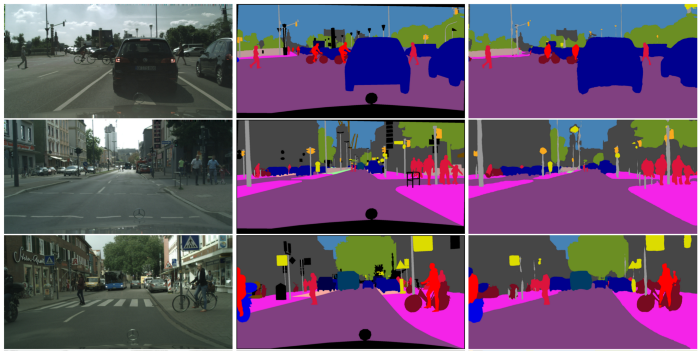
In this article, the authors trained and evaluated using 19 categories from the CityScapes dataset. Through this implementation, you can adjust for any number of outputs required by specific projects.

Below are some validation results of Fast-SCNN compared with the input images and ground truth.