In the world of machine learning, accuracy is crucial. You strive to make your model more accurate by tuning and optimizing parameters, but you can never achieve 100% accuracy. This is the harsh reality of your prediction/classification models; they can never be zero-error. In this article, I will discuss why this happens and other methods to reduce error.
Suppose we observe a response variable Y (qualitative or quantitative) and input variables X with p features or columns (X1, X2…..Xp), and we assume there is a relationship between them. This relationship can be expressed as
Here, f is some fixed but unknown function of X1,…,Xp, and e is a random error term that is independent of X and has an average of zero. In this formula, f represents the systematic information that X provides about Y. The estimation of this relationship or f(X) is called statistical learning.
In general, we cannot perfectly estimate f(X), which leads to an error term known as reducible error. By more accurately estimating f(X) and thereby reducing the reducible error, we can improve the accuracy of the model. However, even if we have a 100% accurate estimate of f(X), our model will still not be error-free, this is known as irreducible error (the e in the equation above).
In other words, irreducible error can be seen as the information that X cannot provide about Y. The loss e may contain unmeasured variables that are useful for predicting Y: since we do not measure them, f cannot be used for prediction. The loss e may also contain unmeasurable variations. For example, for a given patient on a given day, the risk of adverse reactions may vary due to manufacturing variations of the drug itself or the general well-being of the patient on that day.
Such boundary situations exist in every problem, and the errors they introduce are irreducible, as they typically do not exist in the training data. There is nothing we can do about this. What we can do is reduce other forms of error to achieve an almost perfect estimate of f(X). But first, let’s look at other important concepts in machine learning that you need to understand for further learning.
Model Complexity
When learning from a dataset, the complexity of the relationship f(X) between input and response variables is an important factor to consider. Simple relationships are easy to interpret. For example, a linear model looks like this:
It is easy to infer information from this relationship, and it clearly tells how a specific feature affects the response variable. Such models fall into the category of restrictive models because they can only take specific forms, such as linear in this case. However, a relationship may be more complex, for instance, it may be quadratic, circular, etc. Such models are more flexible because they can fit data points more closely and can take different forms. Typically, this approach leads to higher accuracy. But this flexibility comes at the cost of interpretability, as complex relationships are harder to explain.
Choosing a flexible model does not always guarantee high accuracy. This is because our flexible statistical learning programs may try too hard to find patterns in the training data, potentially capturing patterns that are due to random chance rather than the true properties of the unknown function f. This alters our estimate of f(X), leading to less accurate models, a phenomenon known as overfitting.
When inference is the goal, using simple and relatively inflexible statistical learning methods has clear advantages. However, in some cases, we are only interested in prediction, and the interpretability of the predictive model is not a priority at all. In such cases, we will use more flexible methods.
Fit Metrics
To quantify how close the predicted response value is to the true response value for a given observation, the most commonly used metric in regression settings is Mean Squared Error (MSE).
The Mean Squared Error is the average of the squares of the errors or differences between the predicted values and the observed values. If calculated using training data, it is called training MSE; if calculated using test data, it is called test MSE.
For a given value x0, the expected test MSE can always be decomposed into the sum of three basic quantities: the variance of f(x0), the square bias of f(x0), and the variance of the error term e. Here, e is the irreducible error we discussed earlier. So, let’s learn more about bias and variance.
Bias
Bias refers to the error introduced by approximating a potentially very complex real-world problem with a much simpler model. Therefore, if the true relationship is complex, and you try to use linear regression, there will certainly be some bias in estimating f(X). No matter how many observations you have, if you use a simple algorithm in the case of a very complex true relationship, it is impossible to produce accurate predictions.
Variance
Variance refers to the extent to which your estimate of f(X) would change if we used different training datasets to estimate it. Since training data is used to fit statistical learning methods, different training datasets will lead to different estimates. Ideally, the estimates for f(X) should not vary significantly between training sets. However, if a method has high variance, small changes in the training data can lead to large changes in f(X).
General Rule of Bias and Variance
Any change in the dataset will provide a different estimate, and when statistical methods overfit the training dataset, these estimates are very accurate. A general rule is that when statistical methods try to fit the data points more closely, or use more flexible methods, bias decreases, but variance increases.
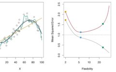
In the image above, on the left, there are charts of three different statistical methods in a regression setting. Yellow represents the linear model, blue represents a slightly nonlinear model, and green represents a highly nonlinear/flexible model, as it overfits the data points. On the right, you can see the chart of the flexibility of these three methods versus MSE. Red represents test MSE, and gray represents training MSE. A method that cannot be determined to have the lowest training MSE will also not necessarily have the lowest test MSE. This is because some methods specifically estimate coefficients to minimize training MSE, but they may not have lower test MSE. This issue can be attributed to overfitting. As shown, the green curve (the most flexible or complex model) has the lowest training MSE but does not have the lowest test MSE. Let’s delve deeper into this issue.
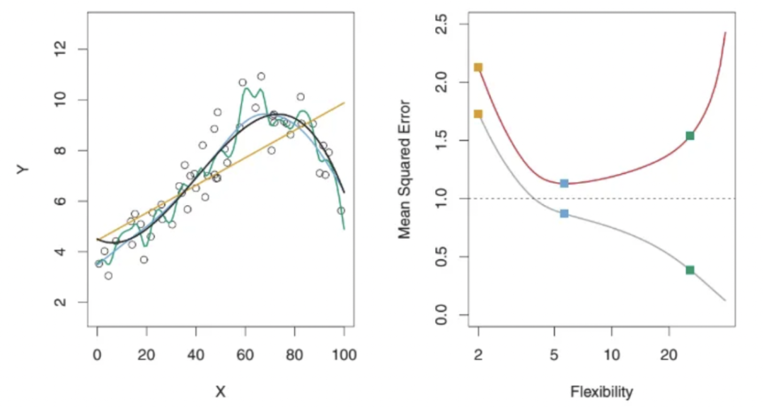
This is a chart showing how test MSE (red curve), bias (green curve), and variance (yellow curve) change with the flexibility of the chosen method for a specific dataset. The lowest MSE point presents an interesting perspective on the error forms of bias and variance. It suggests that as flexibility increases, the rate of decrease in bias is faster than the rate of increase in variance. After a certain point, the bias no longer decreases, but variance starts to increase rapidly due to overfitting.
The implication of flexibility is the complexity of the model, where higher flexibility indicates higher model complexity.
Bias-Variance Tradeoff
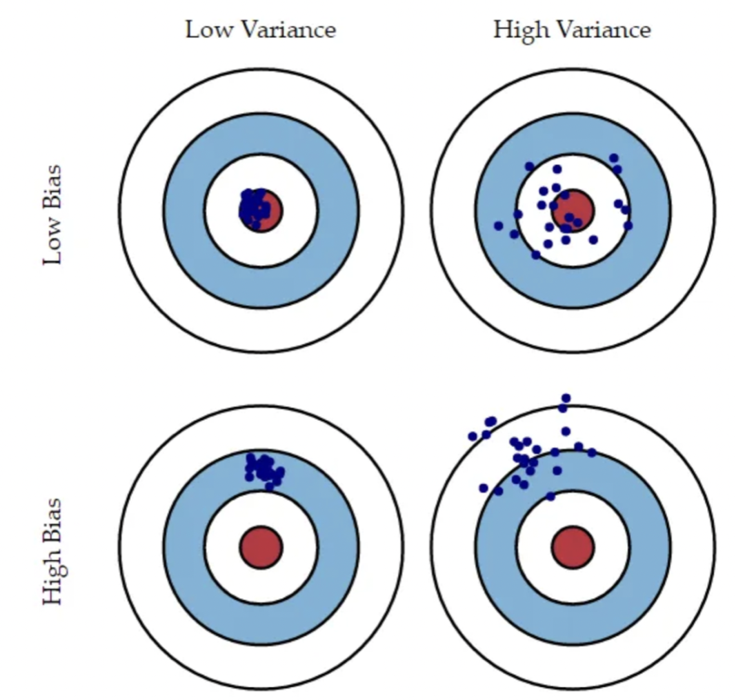
In the above image, imagine the target as a model that perfectly predicts the correct value. The farther we are from the target, the worse our predictions become. Assume we can repeat the entire model-building process to obtain multiple target hit scenarios, where each blue dot represents a different implementation of the model on the same problem based on different datasets. It shows four different situations representing combinations of high bias and low bias as well as high variance and low variance. High bias means all points are far from the target, while high variance means all points are dispersed. This illustration combines previous explanations, making the distinction between bias and variance very clear.
The chart above contains four graphs: the top left shows low bias and low variance, the top right shows low bias and high variance, the bottom left shows high bias and low variance, and the bottom right shows high bias and high variance.
As mentioned earlier, to minimize the expected test error, we need to choose a statistical learning method that achieves both low variance and low bias. There is always a tradeoff between these two values because it is easy to obtain a method with very low bias but high variance (for example, by drawing curves that pass through each training observation point) or a method with very low variance but high bias (by fitting a horizontal line to the data). The challenge is to find a method that has both low variance and low square bias.
The tradeoff between bias and variance is essential for becoming a machine learning champion and is a crucial consideration in the model development process. This concept should be kept in mind when addressing machine learning problems, as it helps improve model accuracy. Maintaining this knowledge also aids you in quickly deciding on the best statistical model in different situations.
If you found this article useful, feel free to scan the code to follow: