In this article, based on the stock price time series data of 20 companies, we will look at four different ways to classify these companies according to the correlation between their stock prices.
Apple (AAPL), Amazon (AMZN), Facebook (META), Tesla (TSLA), Alphabet (Google) (GOOGL), Shell (SHEL), Suncor Energy (SU), ExxonMobil (XOM), Lululemon (LULU), Walmart (WMT), Carters (CRI), Childrens Place (PLCE), TJX Companies (TJX), Victoria’s Secret & Co (VSCO), Macy’s (M), Wayfair (W), Dollar Tree (DLTR), CVS Caremark (CVS), Walgreen (WBA), Curaleaf Holdings Inc. (CURLF)
Our DataFrame df_combined contains the stock prices of the aforementioned companies over 413 days, with no missing data.
Objective
Our goal is to group these companies based on their correlation and examine the validity of these groupings. For instance, Apple, Amazon, Google, and Facebook are typically seen as tech stocks, while Suncor and Exxon are viewed as oil and gas stocks. We will check if we can achieve these classifications using only the correlation between the stock prices of these companies. Using correlation to classify these companies, rather than using stock prices, is crucial; if we used stock prices, companies with similar stock prices would cluster together. However, here we want to classify companies based on the behavior of their stock prices. A simple way to achieve this is to use the correlation between stock prices.
Optimal Number of Clusters
Finding the number of clusters is a question in itself. There are several methods, such as the elbow method, that can be used to find the optimal number of clusters. However, in this work, we attempt to divide these companies into four clusters. Ideally, these four groups should be tech stocks, oil and gas stocks, retail stocks, and others. First, we obtain the correlation matrix of the DataFrame we have.
correlation_mat=df_combined.corr()Define a utility function to display clusters and the companies belonging to those clusters.
# Utility function to print company names and their assigned clusters
def print_clusters(df_combined, cluster_labels):
  cluster_dict = {}
  for i, label in enumerate(cluster_labels):
      if label not in cluster_dict:
          cluster_dict[label] = []
      cluster_dict[label].append(df_combined.columns[i])

  # Print the companies in each cluster -- Follow @public account: Data STUDIO for more quality content
  for cluster, companies in cluster_dict.items():
      print(f"Cluster {cluster}: {', '.join(companies)}")
Method 1: K-means Clustering
K-means clustering is a popular unsupervised machine learning algorithm used to group similar data points based on feature similarity. The algorithm iteratively assigns each data point to the nearest cluster center, then updates the center based on the newly assigned data points until convergence. We can use this algorithm to cluster our data based on the correlation matrix.
from sklearn.cluster import KMeans

# Perform k-means clustering with four clusters
clustering = KMeans(n_clusters=4, random_state=0).fit(correlation_mat)

# Print the cluster labels
cluster_labels=clustering.labels_
print_clusters(df_combined, cluster_labels)

As expected, Amazon, Facebook, Tesla, and Alphabet are clustered together, while oil and gas companies are also grouped together. Additionally, Walmart and Macy’s are clustered together. However, we see some tech stocks, such as Apple, clustered with Walmart.
Method 2: Agglomerative Clustering
Agglomerative clustering is a hierarchical clustering algorithm that iteratively merges similar clusters to form larger clusters. The algorithm starts with individual clusters for each object and then merges the two most similar clusters at each step.
from sklearn.cluster import AgglomerativeClustering

# Perform hierarchical clustering
clustering = AgglomerativeClustering(n_clusters=n_clusters,
                                     affinity='precomputed',
                                     linkage='complete'
                                    ).fit(correlation_mat)

# Display the cluster labels
print_clusters(df_combined, clustering.labels_)

The results differ slightly from those obtained from K-means clustering. We can see some oil and gas companies placed in different clusters.
Method 3: Affinity Propagation Clustering
Affinity propagation clustering is a clustering algorithm that does not require a predetermined number of clusters. It works by sending messages between pairs of data points, allowing the data points to automatically determine the number of clusters and the best cluster assignments. Affinity propagation clustering can effectively identify complex patterns in data, but it is computationally expensive for large datasets.
from sklearn.cluster import AffinityPropagation

# Perform affinity propagation clustering with default parameters
clustering = AffinityPropagation(affinity='precomputed').fit(correlation_mat)

# Display the cluster labels
print_clusters(df_combined, clustering.labels_)

Interestingly, this method finds that four clusters are the optimal number for our data. Additionally, we can observe that oil and gas companies are clustered together, with some tech companies also grouped together.
Method 4: DBSCAN Clustering
DBSCAN is a density-based clustering algorithm that groups points that are closely packed together. It does not require a predetermined number of clusters and can identify clusters of arbitrary shapes. The algorithm is robust to outliers and noise in the data, automatically marking them as noise points.
from sklearn.cluster import DBSCAN

# Removing negative values in correlation matrix
correlation_mat_pro = 1 + correlation_mat

# Perform DBSCAN clustering with eps=0.5 and min_samples=5
clustering = DBSCAN(eps=0.5, min_samples=5, metric='precomputed').fit(correlation_mat_pro)

# Print the cluster labels
print_clusters(df_combined, clustering.labels_)

Here, unlike affinity-based clustering, the DBSCAN method identifies five clusters as the optimal number. It can also be observed that some clusters contain only one or two companies.
Visualization
Simultaneously examining the results of the four clustering methods mentioned above can be useful for gaining deeper insights into their performance. The simplest method is to use a heatmap, with companies on the X-axis and clusters on the Y-axis.
def plot_cluster_heatmaps(cluster_results, companies):
    """
    Plots the heatmaps of clustering for all companies
     for different methods side by side.

    Args:
    - cluster_results: a dictionary of cluster labels for each
       clustering method
    - companies: a list of company names
    - Follow @public account: Data STUDIO for more quality content
    """
    # Extract keys and values from the dictionary
    methods = list(cluster_results.keys())
    labels = list(cluster_results.values())

    # Define heatmap data for each method
    heatmaps = []
    for i in range(len(methods)):
        heatmap = np.zeros((len(np.unique(labels[i])), len(companies)))
        for j in range(len(companies)):
            heatmap[labels[i][j], j] = 1
        heatmaps.append(heatmap)

    # Plot the heatmaps in a 2x2 grid
    fig, axs = plt.subplots(nrows=2, ncols=2, figsize=(12, 12))

    for i in range(len(methods)):
        row = i // 2
        col = i % 2
        sns.heatmap(heatmaps[i], cmap="Blues", annot=True, fmt="g", xticklabels=companies, ax=axs[row, col])
        axs[row, col].set_title(methods[i])

    plt.tight_layout()
    plt.show()

companies=df_combined.columns
plot_cluster_heatmaps(cluster_results, companies)
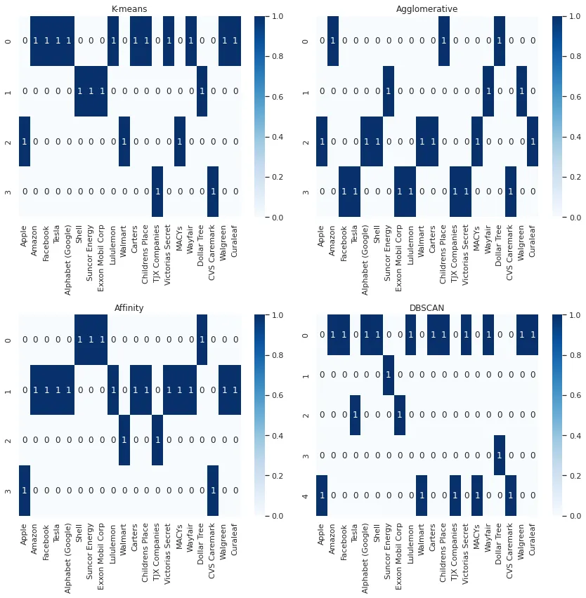
However, when trying to compare the results of multiple clustering algorithms, the aforementioned visualization is not very helpful. Finding a better way to represent this graph would be beneficial.
Conclusion
In this article, we explored four different methods of clustering based on the correlation between the stock prices of 20 companies. The goal was to cluster them in a way that reflects their behavior rather than their stock prices. We tried K-means clustering, Agglomerative clustering, Affinity Propagation clustering, and DBSCAN clustering, each with its own strengths and weaknesses. The results showed that all four methods could cluster companies in a way that aligns with their industry or sector, while some methods had higher computational costs than others. Correlation-based clustering methods provide a useful alternative to price-based clustering methods, allowing for clustering based on company behavior rather than stock prices.