This article is a translated note of the Stanford University CS231N course, authorized by Professor Andrej Karpathy of Stanford University. This is a work of Big Data Digest, and unauthorized reproduction is prohibited. For specific requirements for reproduction, see the end of the article.

Sign up now

Machine Learning Training Registration is now open!
Top-notch instructor course design
Theoretical combined with practical
Four major benefits provided
For detailed introduction, long press the QR code at the end of the article

This is a translated work by Big Data Digest, for specific requirements for reproduction, see the end of the article.

Translation: Han Xiaoyang & Long Xincheng

Editor’s Note:This article is the second series of the Stanford course articles we bring to readers: the fifth issue of the Stanford Deep Learning and Computer Vision Course. The content is from the Stanford CS231N series, for interested readers to experience and learn.

The video translation of this course is also ongoing and will be released soon, please stay tuned!

Big Data Digest will successively release translations and videos, sharing them for free with readers.

We welcome more interested volunteers to join us for communication and learning. All translators are volunteers. If you, like us, are capable and willing to share, please join us. Reply “Volunteer” in the backend of Big Data Digest to learn more.

The Stanford University CS231N course is a classic tutorial in deep learning and computer vision, highly regarded in the industry. Previously, some domestic friends made sporadic translations. To share high-quality content with more readers, Big Data Digest has conducted a systematic and comprehensive translation, and subsequent content will be released successively.

Due to the inability to edit code in the WeChat backend, we used images to present the code. Click on the images for a clearer view.

At the same time, Big Data Digest has previously obtained authorization for the first series of Stanford courses, Stanford University CS224d Course [Machine Learning and Natural Language Processing], which has completed eight sessions. We will continue to push subsequent notes and course videos every Wednesday, please pay attention.

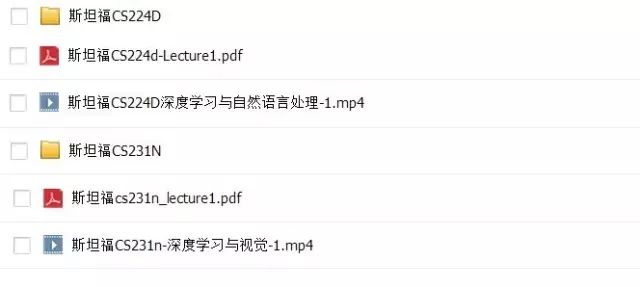
Reply “Stanford” to download the CS231N note PDF version and related video materials

Also obtain related materials for another Stanford series course CS224d Deep Learning and Natural Language Processing

Additionally, for readers interested in further learning and communication, we will organize learning exchanges through QQ groups (due to the limitation of WeChat group members).

Long press the following QR code to directly jump to the QQ group

Or join the group with the number 564538990

◆ ◆ ◆

1.Introduction

Actually, I initially refused to discuss this part of the content because I felt it resembled a summary of advanced mathematics courses. Generally, the intuitive understanding of the backpropagation algorithm is merely a chain rule of derivatives. However, understanding this part and its details is useful for the design and optimization of neural networks, so I reluctantly decided to write about it.

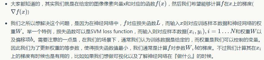
Problem Description and Motivation:

◆ ◆ ◆

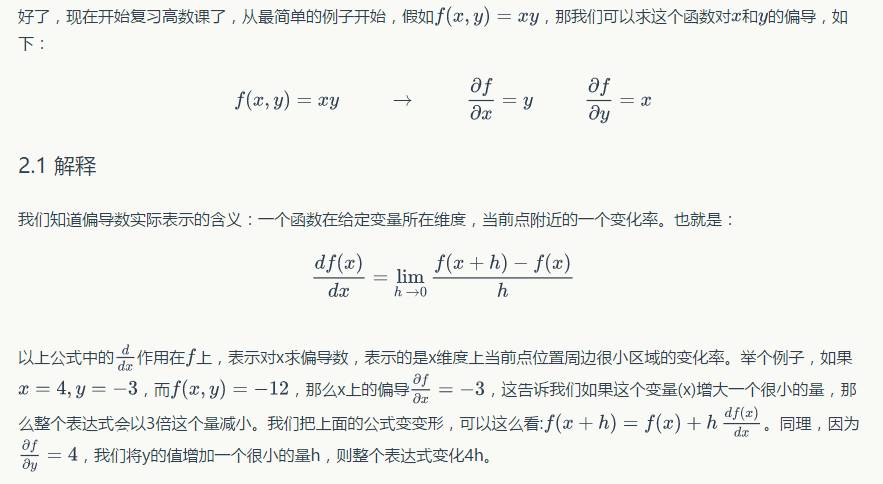
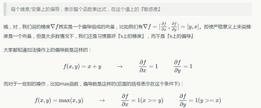
2.Basic Calculus Gradient/Partial Derivative

◆ ◆ ◆

3.Chain Rule of Partial Derivatives for Complex Functions

Consider a slightly more complicated function, for example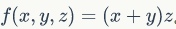Of course, this expression is not that complicated and can be directly differentiated. However, we will use a non-direct approach to help us intuitively understand backpropagation. If we use substitution, we can break the original function into two parts 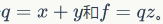For these two parts, we know how to solve their partial derivatives: 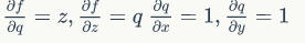Of course, q is a variable we set ourselves, and we are not interested in its partial derivative.

Then the ‘chain rule’ tells us a way to ‘chain’ the above partial derivative formulas to obtain the partial derivatives we are interested in:

Let’s look at an example:

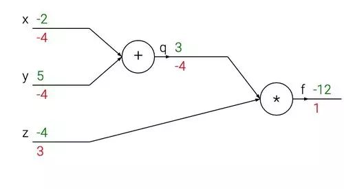
x = -2; y = 5; z = -4

# Forward computation
q = x + y # q becomes 3
f = q * z # f becomes -12

# Pseudo backpropagation:
# First calculated f = q * z
dfdz = q # df/dz = q
dfdq = z # df/dq = z
# Then calculated q = x + y
dfdx = 1.0 * dfdq # dq/dx = 1 Yes, chain rule
dfdy = 1.0 * dfdq # dq/dy = 1

The result of the chain rule is that we are left with the partial derivatives we are interested in [dfdx, dfdy, dfdz], which are the original function’s partial derivatives in terms of x, y, z. This is a simple example, and in the subsequent programs, we will not write out dfdq completely for simplicity, but will use dq instead.

Below is a diagram of this calculation:

◆ ◆ ◆

4.Intuitive Understanding of Backpropagation

In summary: the process of backpropagation is actually a clever process from local to global. For example, in the above circuit diagram, each ‘gate’ can calculate two things after receiving input:

• Output value

• Local gradient corresponding to input and output

Moreover, it is clear that each gate performs this calculation completely independently, without needing to understand the other structures in the circuit diagram. However, after the entire forward transmission process is completed, during the backpropagation process, each gate can gradually accumulate the gradient it contributes to the entire circuit output. The ‘chain rule’ tells us that each gate receives the gradient coming from the back, multiplies it by the local gradient it calculated for each input, and then passes it back.

Taking the above diagram as an example, let’s explain this process. The addition gate receives input [-2, 5] and outputs a result of 3. Since the derivative of the addition operation with respect to both inputs should be 1. The subsequent multiplication part calculates the final result of -12. During the backpropagation process, the chain rule does the following: the output 3 from the addition operation, in the last multiplication operation, receives a gradient of -4. If we anthropomorphize the entire network, we can think of this as the network ‘wanting’ the result of the addition operation to be smaller, and it is trying to decrease it with a strength of 4.

After the addition operation receives this gradient of -4, it multiplies it by the local gradients of both inputs (the derivatives of addition are both 1), resulting in 1 * -4 = -4. If the input x decreases, then the output of the addition gate will also decrease, which will correspondingly increase the output of the multiplication.

Backpropagation can be seen as a ‘dialogue’ between gates in the network, where they ‘want’ their output to be larger or smaller (by how much), so that the final output result is larger.

◆ ◆ ◆

5.Sigmoid Example

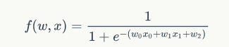
The example above is actually rarely seen in practical applications. Most of the time, the networks and gate functions we encounter are more complex. However, regardless of the complexity, backpropagation can still be used; the only difference is that the layout of the gate functions decomposed from the network may be more complex. Let’s take the previous logistic regression as an example:

This seemingly complex function can actually be seen as a combination of some basic functions, and the partial derivatives of these basic functions are as follows:

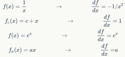
Each of the above basic functions can be seen as a gate. Such a simple combination of elementary functions can accomplish the complex function of the mapping in logistic regression. Below, we draw the neural network and provide specific input-output and parameter values:

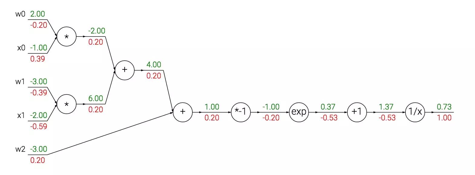
In this diagram, [x0, x1] are the inputs, and [w0, w1, w2] are the adjustable parameters. Therefore, it performs a linear calculation on the input (the inner product of x and w) and then puts the result into the sigmoid function, mapping it to a number between (0,1).

In the above example, the inner product between w and x is decomposed into a long string of small functions, followed by the sigmoid function, Interestingly, the sigmoid function, while seemingly complex, has a simple representation for its derivative, as follows:

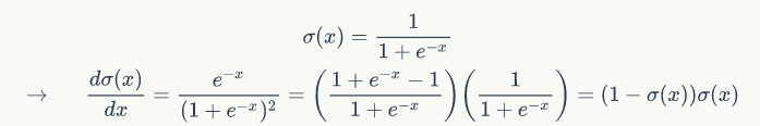
As you can see, its derivative can be simply represented in terms of itself. Therefore, when calculating the derivative, it is very convenient. For example, if the input received by the sigmoid function is 1.0, the output result is -0.73. Then we can easily calculate that its partial derivative is (1-0.73)*0.73~=0.2. Let’s look at the code for the backpropagation calculation in this sigmoid neuron:

w = [2,-3,-3] # We randomly give a set of weights
x = [-1, -2]

# Forward propagation
dot = w[0]*x[0] + w[1]*x[1] + w[2]
f = 1.0 / (1 + math.exp(-dot)) # sigmoid function

# Backpropagation through this sigmoid neuron
ddot = (1 - f) * f # derivative of sigmoid function
dx = [w[0] * ddot, w[1] * ddot] # Backpropagation on the x path
dw = [x[0] * ddot, x[1] * ddot, 1.0 * ddot] # Backpropagation on the w path
# Yes! That's how it's done! Isn't it simple?

5.1 Engineering Implementation Tips

Looking back at the code above, you will find that when actually implementing the code, there is a technique that can help us easily implement backpropagation. We will decompose the forward propagation process into parts that can be easily traced back during backpropagation.

◆ ◆ ◆

6.Backpropagation in Practice: Complex Functions

Let’s look at a slightly more complex function:

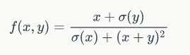
By the way, this function has no practical significance. We mention it only to provide an example of how to use backpropagation for complex functions. If you directly differentiate this function with respect to x or y, you will get a very complex form. However, if you use backpropagation to compute the specific gradient values, you won’t have this trouble. We can decompose this function into small parts, perform forward and backpropagation calculations, and get the results. The code for the forward propagation calculation is as follows:

x = 3 # example
y = -4

# Forward propagation
sigy = 1.0 / (1 + math.exp(-y)) # Sigmoid function on a single value
num = x + sigy 
sigx = 1.0 / (1 + math.exp(-x)) 
xpy = x + y      
xpysqr = xpy**2                 
den = sigx + xpysqr
invden = 1.0 / den                                       
f = num * invden # Done!                                

Note that we did not calculate the final result of forward propagation at once, but deliberately left many intermediate variables. These are simple expressions for which we can directly compute local gradients. Therefore, calculating backpropagation becomes simple: we look back from the final result, and we will use each intermediate variable sigy, num, sigx, xpy, xpysqr, den, invden from the forward operation. We will multiply the gradient values coming back by them to obtain the partial derivatives for backpropagation. The code for the backpropagation calculation is as follows:

# Local function expression is f = num * invden
dnum = invden                               
dinvden = num    
# Local function expression is invden = 1.0 / den 
dden = (-1.0 / (den**2)) * dinvden                            
# Local function expression is den = sigx + xpysqr
dsigx = (1) * dden
dxpysqr = (1) * dden
# Local function expression is xpysqr = xpy**2
dxpy = (2 * xpy) * dxpysqr                                        #(5)
# Local function expression is xpy = x + y
dx = (1) * dxpy                                                    
dy = (1) * dxpy                                                    
# Local function expression is sigx = 1.0 / (1 + math.exp(-x))
dx += ((1 - sigx) * sigx) * dsigx # Note that we use += here!!
# Local function expression is num = x + sigy
dx += (1) * dnum                                                  
dsigy = (1) * dnum                                                
# Local function expression is sigy = 1.0 / (1 + math.exp(-y))
dy += ((1 - sigy) * sigy) * dsigy                                 
# Done!

When implementing actual programming, pay attention to the following:

• When calculating forward propagation, be sure to retain some intermediate variables: In backpropagation calculations, some results from forward propagation calculations will be used again. This can greatly speed up backpropagation calculations.

6.1 Common Patterns in Backpropagation Calculations

Even though the structure of the neural network built and the neurons used may differ, in most cases, the gradient calculations in backpropagation can be categorized into a few common patterns. For example, the three most common simple operation gates (addition, multiplication, maximum) have very simple and straightforward roles in backpropagation calculations. Let’s take a look at the simple neural network below:

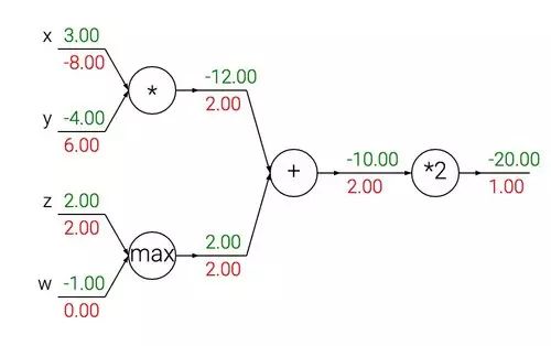
The above figure contains the three gates we mentioned: add, max, and multiply.

• The addition gate in backpropagation calculations distributes the gradient it receives uniformly to both input paths, regardless of the input values, since the derivative of addition is +1.0.

• The max (maximum) gate, unlike the addition gate, only passes the gradient back to one input path during backpropagation calculations. This is because the derivative of max(x,y) is +1.0 for the larger number among x and y, while the derivative for the smaller number is 0.

• The multiplication gate is even easier to understand, as the derivative of x*y with respect to x is y, and with respect to y is x. Therefore, in the above figure, the gradient on x is -8.0, that is, -4.0*2.0.

Due to the nature of gradient backpropagation, neural networks are very sensitive to input. Let’s take the multiplication gate as an example. If all inputs are scaled by 1000 times while keeping the weights w unchanged, then during backpropagation calculations, the gradient received on the x path remains unchanged, while the gradient on w will increase by 1000 times. This forces you to reduce the learning rate to 1/1000 to maintain balance. Therefore, preprocessing input data is also very important in many neural network problems.

6.2 Vectorized Gradient Operations

All the parts above deal with single-variable functions. In practice, when handling many data (such as image data), the dimensions are often high. In this case, we need to extend the single-variable function backpropagation to vectorized gradient operations. It is crucial to pay attention to the dimensions of each matrix in matrix operations and transpose operations.

We can extend forward and backpropagation operations through simple matrix operations. Example code is as follows:

# Forward propagation operation
W = np.random.randn(5, 10)
X = np.random.randn(10, 3)
D = W.dot(X)

# Suppose we have now obtained the gradient dD back to D
dD = np.random.randn(*D.shape) # Same dimension as D
dW = dD.dot(X.T) # .T operation calculates transposition, dW is the gradient on the W path
dX = W.T.dot(dD)  # dX is the gradient on the X path

◆ ◆ ◆

7.Conclusion

Intuitively, backpropagation can be seen as the chain rule of derivatives illustrated graphically. Finally, we use a set of diagrams to illustrate the forward propagation and backward residual propagation processes during actual optimization:

About Reproduction

For reproduction, please prominently indicate the author and source at the beginning of the article (Reproduced from: Big Data Digest | bigdatadigest), and place a prominent QR code of Big Data Digest at the end of the article. For articles without original markings, please edit according to reproduction requirements; they can be directly reproduced. After reproduction, please send us the link. For articles with original markings, please send [Article Name - WeChat Public Account Name and ID] to apply for whitelist authorization. Unauthorized reproduction and adaptations will be legally pursued. Contact email: [email protected].

◆ ◆ ◆

Big Data Articles Stanford Deep Learning Course

Reply “Volunteer” in the backend of Big Data Digest to learn how to join us

Column Editor

Project Management

Content Operation: Wei Zimin

Coordination: Wang Decheng

Previous wonderful article recommendations, click the image to read

[Another Heavyweight] Authorized for Translation Again, Stanford CS231N Deep Learning and Computer Vision

Stanford Deep Learning Course Volume 7: RNN, GRU, and LSTM

Stanford CS231N Deep Learning and Computer Vision Volume 2: Image Classification and KNN