MLNLP community is a well-known machine learning and natural language processing community both domestically and internationally, covering NLP master’s and doctoral students, university teachers, and industry researchers.
The vision of the community is to promote communication and progress between the academic and industrial circles of natural language processing and machine learning, especially for beginners.
Reprinted from | Beijing University of Posts and Telecommunications GAMMA Lab
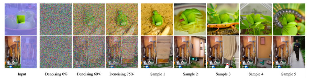
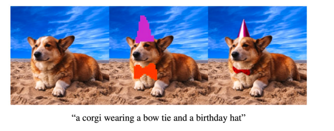
1. Applications of Diffusion Models
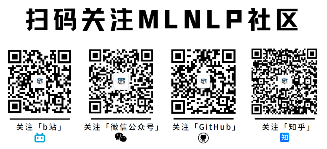
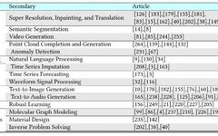
Diffusion models have extensive research and applications in computer vision, natural language processing, and other fields. The following image shows some studies and applications of diffusion models in different domains.
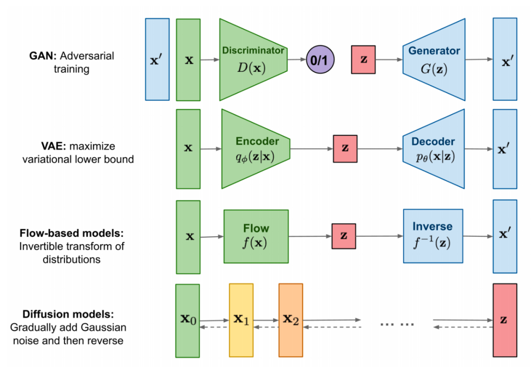
2. Comparison of Diffusion Models with Other Models
The inspiration for diffusion models comes from non-equilibrium thermodynamics. The diffusion model defines a diffusion Markov chain and slowly adds random noise to the data, then learns the reverse diffusion process to construct the desired data samples from the noise. Unlike VAE or flow models, diffusion models are learned through a fixed process, and the variables during the diffusion process have the same dimension as the original variables.
2.1 Comparison of VAE and Diffusion Models
Variational autoencoders aim to learn encoders and decoders to map input data to values in a continuous latent space. In these models, embeddings can be interpreted as latent variables in probabilistic generative models, and probabilistic decoders can be represented by parameterizing the likelihood function. Furthermore, it is assumed that data x is generated by some unobserved latent variables z using conditional distributions, and is used to approximate inference z. To ensure effective inference, we use variational Bayesian methods to maximize the evidence lower bound:
DDPM can be viewed as a multi-layer Markov VAE. The forward process represents the encoder, while the reverse process represents the decoder. Additionally, DDPM shares the decoder across multiple layers, and all latent variables are the same size as the sample data. Under continuous time conditions, optimizing the diffusion model can be seen as training an infinite, deep, multi-layer VAE. This demonstrates that diffusion models can be interpreted as the continuous limit of hierarchical VAEs.
2.2 Derivation Process of Diffusion Models
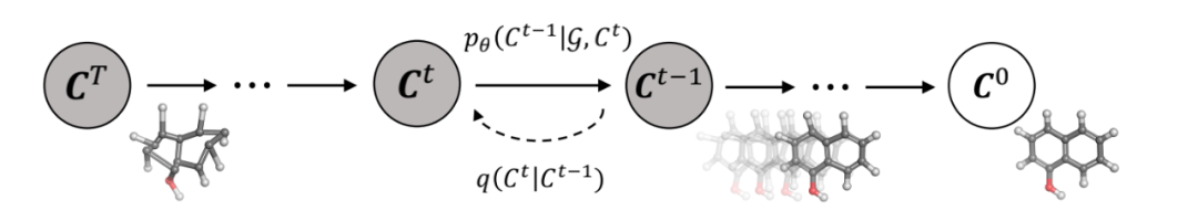
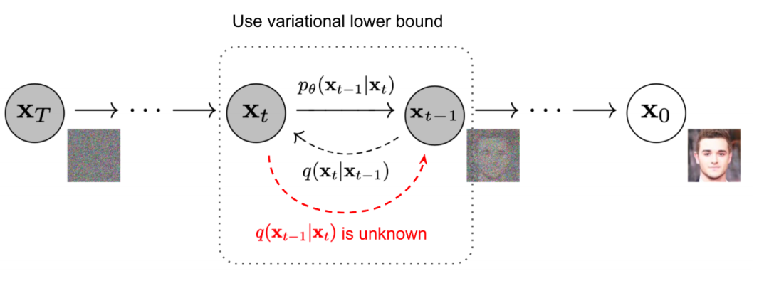
Diffusion models consist of two processes: the forward process and the reverse process, where the forward process is also known as the diffusion process, as shown in the figure below. Both the forward and reverse processes are parameterized Markov chains, where the reverse process can be used to generate data, and we will model and solve this through variational inference.
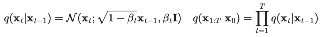
Forward Process: Given a data point sampled from the real data distribution. We define the forward diffusion process, which adds Gaussian noise over steps, generating a series of noisy samples. The step size is controlled by .
As increases, it gradually loses its identifiable features. At that time, it conforms to an isotropic Gaussian distribution.
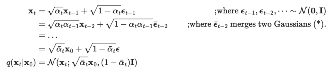
A good property of the diffusion process is that at any time, it can be obtained using the reparameterization trick. Moreover,
Reverse Process: If we can reverse the above process and from , we can reconstruct real samples from the input Gaussian noise (). Note that if is sufficiently small, then it is also Gaussian distributed. However, we cannot estimate because it requires information from the entire dataset. Therefore, we need to learn to approximate this conditional probability so that we can complete the reverse diffusion.
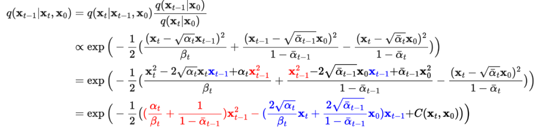
When given , the reverse conditional probability is known:
where is the equation that is not included. Thus it can be ignored.
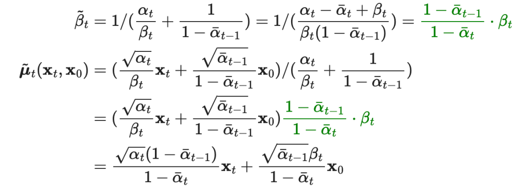
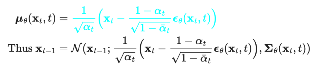
So the mean and variance are
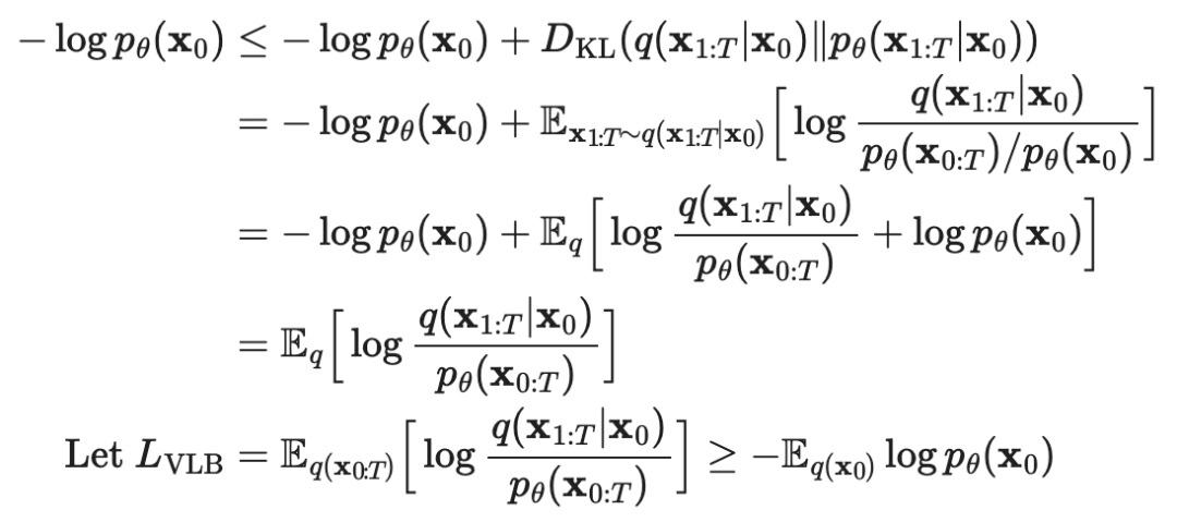
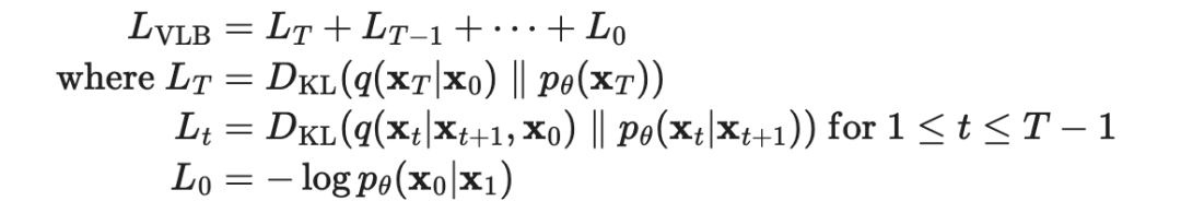
We can optimize the negative log-likelihood function
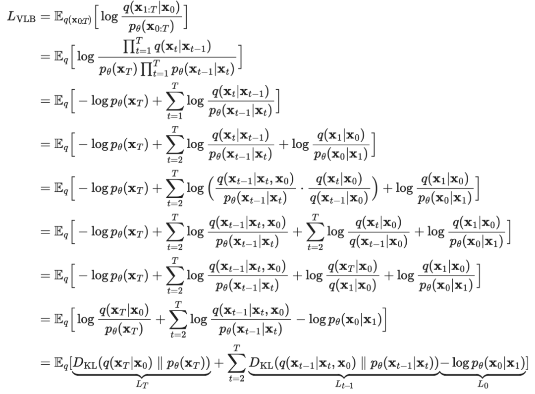
which can be further written as
each component can be rewritten as
where is a constant that can be ignored, and can be seen as pulling two distributions and closer.
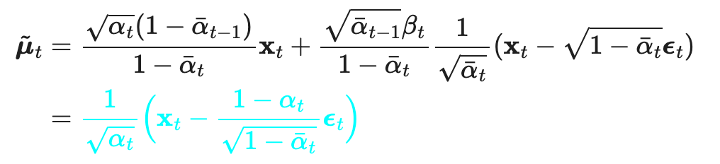
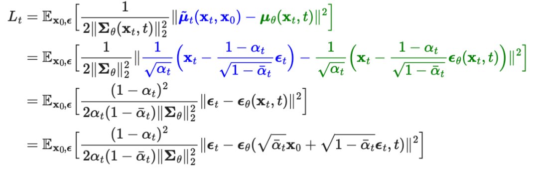
We need to use neural networks to approximate the conditional probability of reverse diffusion, resulting in , we train to predict . Because is known during the training process, it can be predicted through .
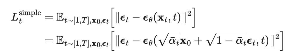
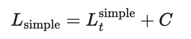
Furthermore, simplifying reveals that ignoring the weight term improves the training process
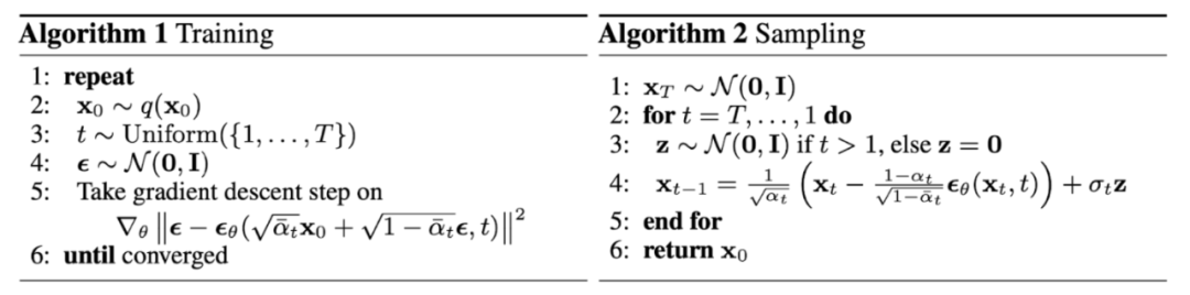
The training process can be seen as:
-
Getting input, randomly sampling a .
-
Sampling noise from a standard Gaussian distribution.
-
Technical Group Invitation

△ Long press to add assistant
Scan the QR code to add the assistant WeChat
Please note: Name – School/Company – Research Direction
(For example: Xiaozhang – Harbin Institute of Technology – Dialogue System)
You can apply to join Natural Language Processing / Pytorch and other technical groups
About Us
MLNLP community is a grassroots academic community built by machine learning and natural language processing scholars from both domestic and international backgrounds. It has developed into a well-known community in the field of machine learning and natural language processing, aiming to promote progress among academics, industry professionals, and enthusiasts.
The community can provide an open communication platform for practitioners in further education, employment, and research. Everyone is welcome to follow and join us.