Author: Eryk Lewinson

Translator: Wang Anxu
Proofreader: zrx




This article is approximately 4400 words long and is recommended for a 5-minute read.
This article explores three methods of creating meaningful features using time-related information.

Tags: Time Frame, Machine Learning, Python, Technical Demonstration

Imagine you are starting a new data science project. The goal is to build a model to predict the target variable Y. You have received some data from stakeholders/data engineers, conducted thorough EDA, and selected some variables that you believe are relevant to the problem at hand. Then, you finally build your first model. The score is acceptable, but you believe you can do better. What should you do?Here you can follow up in many ways. One possibility is to increase the complexity of the machine learning model you are using. Alternatively, you could try to come up with some more meaningful features and continue using the current model (at least for now).For many projects, business data scientists and participants in data science competitions like Kaggle believe that the latter—identifying more meaningful features from the data—can often maximize model accuracy with minimal effort.You are effectively shifting complexity from the model to the features. Features don’t necessarily have to be very complex; ideally, we would find features that have a strong and simple relationship with the target variable.Many data science projects include some information about time changes, which is not limited to time series forecasting problems. For example, you often find these features in traditional regression or classification problems. This article explores how to create meaningful features using date-related information. We propose three methods, but we need to do some preparation first.

Setup and Data

In this article, we will use some well-known Python packages more often, but we also use a relatively obscure package, scikit-lego. It is a library that contains many useful features that extend the capabilities of scikit-learn. We import the necessary libraries:

For simplicity, we will generate the data ourselves. In this example, we use an artificial time series. First, we create an empty DataFrame that spans four calendar years (using pd.date_range). Then we create two columns:

• day_nr – a numerical index representing the passage of time;

• day_of_year – the day of the year;

Finally, we need to create the time series itself. To do this, we combine two transformed sine curves with some random noise. The code used to generate the data is based on the code included in the scikit-lego documentation.https://scikit-lego.readthedocs.io/en/latest/

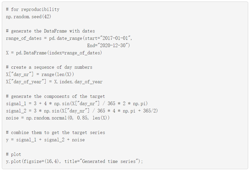
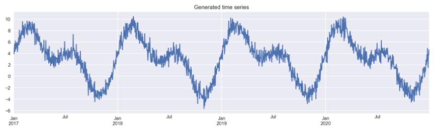
Figure 1: Generated Time SeriesThen, we create a new DataFrame to store the generated time series. This DataFrame will be used to compare model performance using different feature engineering methods.

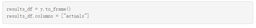
Creating Time-Related FeaturesIn this section, we describe three methods for generating time-related features. Before diving deeper, we should define an evaluation framework. The simulated data contains observations over a period of four years. We use the data generated from the first three years as the training set and evaluate in the fourth year. In this process, the Mean Absolute Error (MAE) will be used as the evaluation metric. Below we define a variable to separate these two sets:

Method #1: Dummy Variables

We will start with something you may already be familiar with. The simplest way to encode time-related information is to use dummy variableshttps://en.wikipedia.org/wiki/Dummy_variable_(statistics) (also known as one-hot encoding). Let’s look at an example. Below you can see the output of our operation.

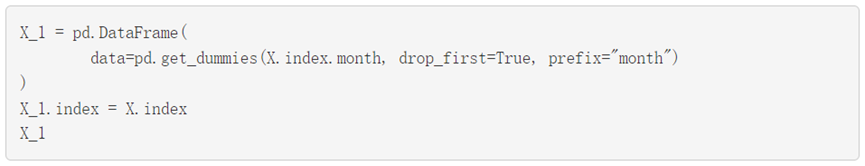
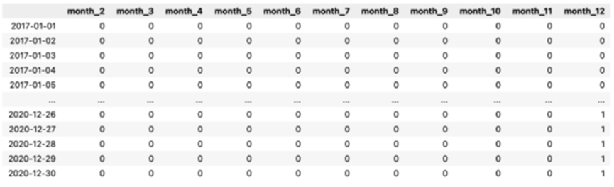
Table 1: DataFrame with Month Dummy VariablesFirst, we extracted information about the month from the DatetimeIndex (encoded as integers in the range of 1 to 12). Then, we used the pd.get_dummies function to create dummy variables. Each column contains information about whether the observation (row) comes from a given month. You may have noticed that we dropped one level, and now there are only 11 columns. This is done to avoid the well-known dummy variable trap (perfect multicollinearity). In our example, we used the dummy variable method to capture the month in which the observations were recorded. The same method can be used to indicate a range of other information from the DatetimeIndex. For example, the day/week/quarter of the year, whether a given date is a weekend, the first/last day of a period, etc. You can find a list of all possible features we can extract frompandashttps://pandas.pydata.org/pandas-docs/stable/user_guide/timeseries.html#time-date-components documentation index. Tip:This goes beyond simple exercises, but in real-life scenarios, we can also use information about special days (e.g., public holidays, Christmas, Black Friday, etc.) to create features. The holidays library is a nice Python library that contains information about past and future special days for each country. As mentioned in the introduction, the goal of feature engineering is to shift complexity from the model side to the feature side. This is why we will use one of the simplest ML models, “linear regression,” to see how well we can fit the time series using only the created dummy model.

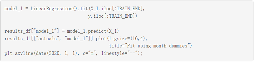
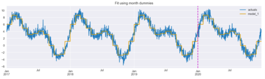
Figure 2: Fitting with Month Dummy Variables. The vertical line separates the training set and test set.We can see that the fitted line follows the time series quite well, although it is somewhat jagged (stair-step) — this is due to the discontinuity of the dummy features. We will attempt to solve this issue with the following two methods. It is worth mentioning that when using nonlinear models such as decision trees (or their ensembles), we do not explicitly encode features like month number or a specific day of the year as dummy variables. These models can learn non-monotonic relationships between ordinal input features and the target.

Method #2: Cyclical Encoding Using Sine/Cosine Transformations

As we saw earlier, the fitted line resembles a step function. This is because each dummy variable is treated separately, resulting in a lack of continuity. However, variables like time have apparent periodic continuity. Imagine we are dealing with energy consumption data. It makes sense that there is a stronger connection between observed consumption in consecutive months. Following this logic, the connection between December and January, as well as between January and February, is strong. In contrast, the connection between January and July is not as close. This similarly applies to other time-related information. So how can we incorporate this knowledge into feature engineering? Trigonometric functions provide one way.We can use the following sine/cosine transformations to encode cyclical time features into two features.

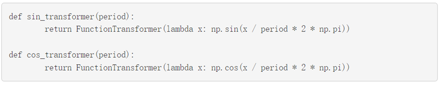
In the code snippet below, we copy the initial DataFrame, add a column with the month number, and then encode the month and day_of_year columns using sine/cosine transformations. Next, we plot two pairs of curves.

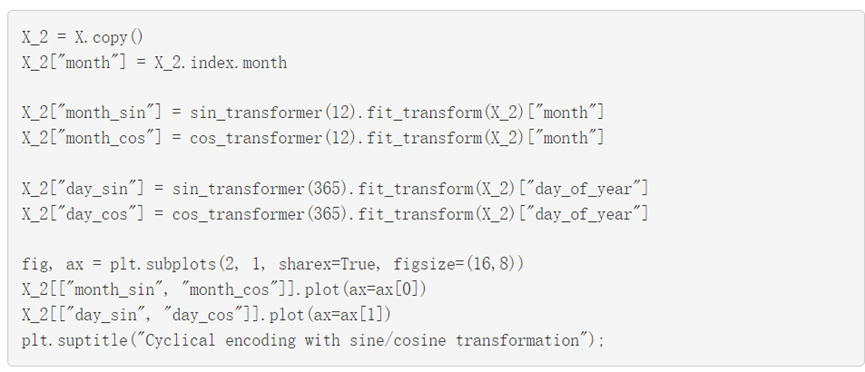
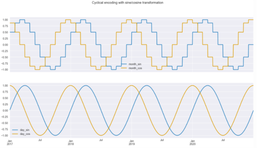
Figure 3: Sine/Cosine Transformations Based on Month and Daily SequenceAs shown in Figure 3, we can draw two conclusions from the transformed data: first, we can see that when using month encoding, the curves are step-like, but when using daily frequency, the curves are smoother; second, we can also see that we must use two curves instead of one. Due to the periodicity of the curves, if you draw a horizontal line within a year, you will intersect the curves at two places. This is not sufficient for the model to understand the time point of the observations. However, with these two curves, there is no such issue, and the user can identify each time point. This is clearly visible when we plot the values of the sine/cosine functions on a scatter plot. In Figure 4, we can see a circular pattern without overlapping values.

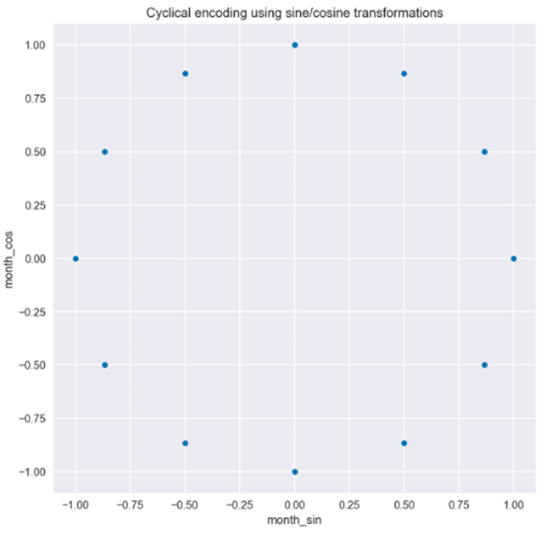
Figure 4: Scatter Plot of Sine/Cosine TransformationsWe will fit the same linear regression model using only the newly created features from the daily frequency.

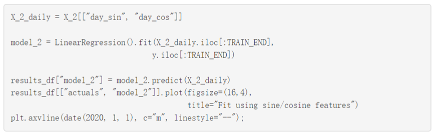
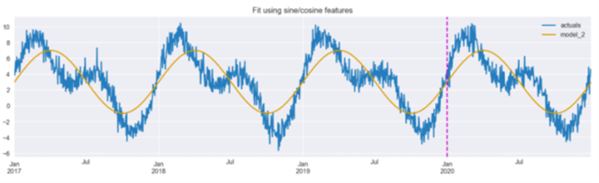
Figure 5: Fitting with Sine/Cosine Transformations. The vertical line separates the training set and test set.Figure 5 shows that the model is able to capture the overall trend of the data, identifying periods of higher and lower values. However, the magnitude of the predictions seems less accurate, and at first glance, this fit appears worse than the fit achieved using dummy variables (Figure 2). Before we discuss the third feature engineering technique, it is worth mentioning that this method has a serious drawback that becomes apparent when using tree-based models. By design, tree-based models split based on individual features. As we mentioned earlier, sine/cosine features should be considered together to correctly identify time points over a period.

Method #3: Radial Basis Functions

The final method uses radial basis functions. We will not go into detail about their actual meaning, but you can read more about the topic herehttps://en.wikipedia.org/wiki/Radial_basis_function. Essentially, we want to address the issue we encountered in the first method, which is that time features have continuity. We use the convenient scikit-lego library, which provides the RepeatingBasisFunction class and specifies the following parameters:

• The number of basis functions we want to create (we chose 12).

• The column used to index the RBF. In our example, this is the column containing information about which day of the year a given observation comes from.

• The range of inputs—in our example, the range is from 1 to 365.

• How to handle the remaining columns of the DataFrame we will use to fit the estimator. “drop” will only keep the created RBF features, while “passthrough” will retain both the new and old features.

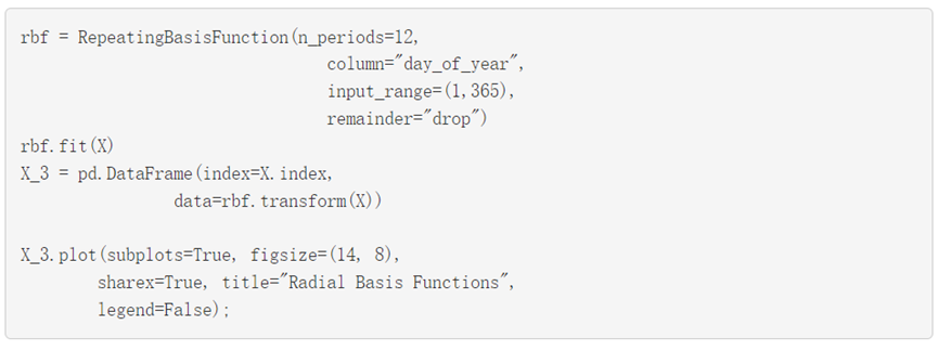
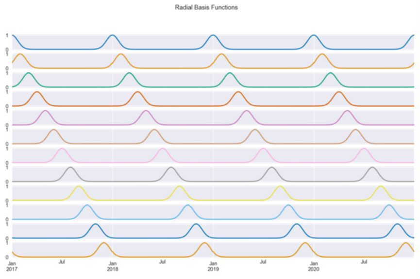
Figure 6: 12 Radial Basis FunctionsFigure 6 shows the 12 radial basis functions created using days as input. Each curve contains information about how close we are to a given day of the year (since we chose that column). For example, the first curve measures the distance from January 1st, thus peaking on the first day of each year and symmetrically decreasing as we move away from that date. By design, the basis functions are evenly distributed within the input range. We chose 12 because we want the RBF to resemble months. Thus, each function will roughly show (due to the varying lengths of months) the distance to the first day of that month. Similar to the previous methods, let’s fit a linear regression model using the 12 RBF features.

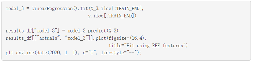
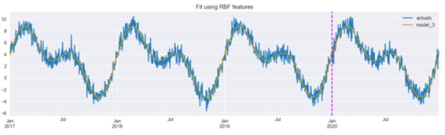
Figure 7: Fitting with Radial Basis Functions. The vertical line separates the training set and test set.Figure 7 shows that the model is able to accurately capture the real data when using RBF features. When using radial basis functions, we can adjust two key parameters:

• The number of radial basis functions;

• The shape of the bell curve—this can be modified using the width parameter of the RepeatingBasisFunction.

One way to adjust these parameter values is to use grid search to identify the best values for a given dataset.

Final Comparison

We can execute the following code snippet to generate values and compare the different methods of encoding time-related information.

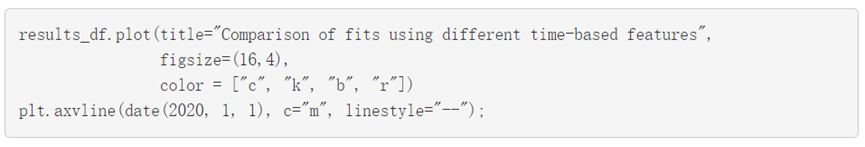
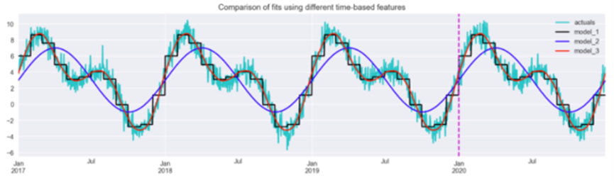
Figure 8: Model Fit Comparisons Using Different Time-Based Features. The vertical line separates the training set and test set.Figure 8 illustrates that radial basis functions are closest to the methods considered. Sine/cosine features allow the model to pick up the main patterns but are insufficient to fully capture the dynamics of the series. Using the code snippet below, we calculate the Mean Absolute Error for each model on the training and test sets. We expect the scores between the training and test sets to be very similar because the generated series is almost completely periodic—the only difference between years is the random component. Of course, this is not the case in real life, where we encounter more variability over the same periods over time. However, we will also use many other features (e.g., some measure of trend or the passage of time) to explain these variations.

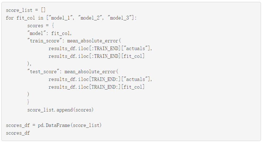
As before, we can see that the model using RBF features achieved the best fit, while the fit using sine/cosine features was the worst. Our assumption about the similarity of scores between the training and test sets was also confirmed.

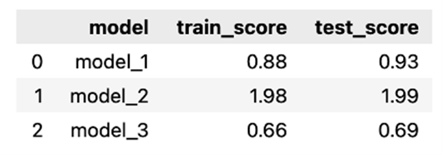
Table 2: Comparison of Scores (MAE) from Training/Test Sets

Key Points

• We have demonstrated three methods to encode time-related information as features for machine learning models.

• In addition to the most popular dummy encoding, there are other methods that are better suited for encoding the cyclical nature of time.

• The granularity of the time intervals is very important for the shape of the newly created features.

• Using radial basis functions, we can decide on the number of functions to use and the width of the bell curve.

You can find the code used in this article on my GitHub https://github.com/erykml/nvidia_articles/blob/main/three_approaches_to_encoding_time_information_as_features_for_ml_models.ipynb.

References:

https://scikit-learn.org/stable/auto_examples/applications/plot_cyclical_feature_engineering.htmlhttps://scikit-lego.readthedocs.io/en/latest/preprocessing.htmlhttps://pandas.pydata.org/pandas-docs/stable/user_guide/timeseries.html#time-date-components Original Title:Three Approaches to Encoding Time Information as Features for ML ModelsOriginal Link:https://developer.nvidia.com/blog/three-approaches-to-encoding-time-information-as-features-for-ml-models/Editor: Huang Jiyan

Translator’s Profile

Wang Anxu, a graduate student at Nanjing University of Aeronautics and Astronautics. Interested in data science, eager to improve through sharing and learning new knowledge in practice. Enjoys watching movies and reading novels in leisure time. Loves making new friends and exploring new hobbies together.

Translation Team Recruitment Information

Job Content: Requires a meticulous heart to translate selected foreign articles into fluent Chinese. If you are an international student in data science/statistics/computer science or working overseas in related fields, or if you are confident in your language skills, please join the translation team.

What You Can Get: Regular translation training to improve volunteers’ translation skills, enhance awareness of cutting-edge data science, and overseas friends can stay connected with domestic technical application development. The THU Data Team’s background provides good development opportunities for volunteers.

Other Benefits: Data scientists from well-known companies, students from prestigious universities such as Peking University and Tsinghua University, as well as overseas students will become your partners in the translation team.

Click “Read the Original” at the end to join the Data Team~

Reprint Notice

If you need to reprint, please indicate the author and source prominently at the beginning (transferred from: Data Team ID: DatapiTHU), and place a prominent QR code of Data Team at the end of the article. For articles with original identification, please send [Article Name – Pending Authorization Public Account Name and ID] to the contact email to apply for whitelist authorization and edit as required.

After publishing, please provide the link feedback to the contact email (see below). Unauthorized reprints and adaptations will be pursued legally.

Click “Read the Original” to embrace the organization