The Victory of ChatGPT: A Triumph of Probability Theory and Bayes’ Theorem

● 　● 　●

Probability Theory and Bayes

Regarding probability theory, the Frenchman known as the Newton of probability, Laplace (1749-1827), once said:

“This science, originating from gambling, will become one of the most important parts of human knowledge; most problems in life will simply be problems of probability.”

Over two hundred years later, modern civilization has confirmed Laplace’s prophecy. This world is full of uncertainty, with probabilities everywhere; everything is random. Without abstract definitions, the basic intuitive concepts of probability theory have already permeated people’s work and lives, from the lottery tickets that everyone can buy to the stars in the universe, and the complexities of computers and artificial intelligence, all closely related to probability.

So, who is Bayes?

Thomas Bayes (1701-1761) was an 18th-century British mathematician and statistician who was once a pastor. However, he was “unknown during his lifetime but worshipped after his death”. He became popular in the contemporary scientific community primarily due to the famous Bayes’ theorem named after him. This theorem not only historically facilitated the development of the Bayesian school but is now widely applied in machine learning, which is closely related to artificial intelligence.【2】.

What did Bayes do? He studied a probability problem involving “white balls and black balls”. Probability problems can be calculated forward or backward. For example, if there are 10 balls in a box, with two colors (black and white), and we know that there are 5 white and 5 black, then if I ask you the probability of randomly picking a black ball, the answer is obviously 50%! If there are 6 white and 4 black, then the probability of picking a black ball would be 40%. Now consider a more complex case: if there are 2 white and 8 black balls, what is the probability of randomly picking 2 balls and getting 1 black and 1 white? The total number of ways to pick 2 balls from 10 is 10*9=90, and there are 16 ways to get 1 black and 1 white, so the probability is 16/90, approximately 17.5%. Therefore, by performing some simple combinatorial calculations, we can calculate the probability of picking n balls, of which m are black, under various distributions of the 10 balls. These are all examples of forward probability calculations.

However, Bayes was more interested in the reverse probability problem: Suppose we do not know the ratio of black to white balls in the box; we only know there are a total of 10 balls. For instance, if I randomly pick 3 balls and find 2 black and 1 white, the reverse probability problem is to guess the ratio of black to white balls in the box based on this sample (2 black and 1 white).

This can also be illustrated with the simplest coin toss experiment. Suppose we do not know if the coin is fair, meaning we do not know the physical bias of the coin. In this case, the probability p of getting heads may not equal 50%. The reverse probability problem attempts to guess the value of p from one or more experimental samples.

To solve the reverse probability problem, Bayes provided a method in his paper, namely Bayes’ theorem:

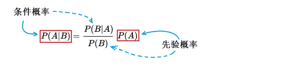
P(A|B) = (P(B|A) * P(A)) / P(B) (1)

Here, A and B are two random events, P(A) is the probability of A occurring; P(B) is the probability of B occurring. P(A|B) and P(B|A) are called conditional probabilities: P(A|B) is the probability of A occurring given that B has occurred; P(B|A) is the probability of B occurring given that A has occurred.

Examples of Applying Bayes’ Theorem

Bayes’ theorem can be interpreted from two angles: one is “it describes the mutual influence of two random variables A and B”; the other is “how to revise the prior probability to obtain the posterior probability”. The following examples illustrate this.

Firstly, in brief, Bayes’ theorem (1) involves two random variables A and B, representing the relationship between the two conditional probabilities P(A|B) and P(B|A).

Example 1: In a small town, the security was not very good in January, with 6 cases of burglary occurring in 30 days. The police station has an alarm system that goes off during incidents, including natural disasters like fires and storms, as well as human disasters like theft and rape. In January, the alarm went off every day. Based on past experience, if a resident is burglarized, the probability of the alarm going off is 0.85. Now, people hear the alarm again; what is the probability that this alarm indicates a burglary?

Let’s analyze this problem. A: burglary; B: alarm. Then, we know (in January):

The probability of burglary P(A) = 6/30 = 0.2; the probability of the alarm going off P(B) = 30/30 = 1; P(B|A) = the probability of the alarm going off during a burglary = 0.85.

So, according to formula (1), substituting the known three probabilities gives P(A|B) = (0.85 * 0.2 / 1) = 0.17.

This means the probability that “the reason for the alarm going off is due to a burglary” is 17 percent.

Next, let’s illustrate how to use Bayes’ theorem to calculate the “posterior probability” from the “prior probability”. First, we rewrite (1) as follows:

(2)

To summarize (2) in one sentence, it states: Using the new information brought by B occurring, we can modify the “prior probability” P(A) when B has not occurred to obtain the “posterior probability” P(A|B) when B occurs (or exists).

First, let’s use an example given by American psychologist and 2002 Nobel Prize winner Daniel Kahneman to illustrate.

Example 2: In a city, there are two colors (blue and green) of taxis: the ratio of blue to green taxis is 15:85. One day, a blue taxi had an accident and fled the scene, but there was a witness who identified the taxi as blue. However, how credible is the witness? The police conducted a “blue-green” test under the same conditions and found that the witness identified correctly 80% of the time and incorrectly 20% of the time. The question is to calculate the probability that the fleeing taxi was blue.

Let A = the taxi is blue, B = the witness saw blue. First, we consider the basic ratio of blue and green taxis (15: 85). This means that without the witness, the probability that the fleeing taxi is blue is 15%, which is the “prior probability” P(A) = 15%.

Now, with a witness, the probability of event A occurring has changed. The witness saw the taxi as “blue”. However, the witness’s ability to identify also needs to be discounted, with only an accuracy of 80%, which is also a random event (denoted as B). Our question is to find the probability that the fleeing taxi is “truly blue” given the condition that the witness “saw a blue taxi”, i.e., the conditional probability P(A|B). The latter should be greater than the prior probability of 15%, because the witness saw a “blue taxi”. How do we revise the prior probability? We need to calculate P(B|A) and P(B).

Since P(B|A) is the probability of “seeing blue” given that “the taxi is blue”, we have P(B|A) = 80%. The calculation of probability P(B) is a bit more complicated. P(B) refers to the probability that the witness saw a taxi as blue, which should equal the sum of two situations: one is the taxi being blue and the identification being correct; the other is the taxi being green and being misidentified as blue.

Thus:P(B) = 15% × 80% + 85% × 20% = 29%

Using Bayes’ formula:

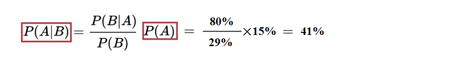
We can calculate that the probability that the fleeing vehicle is blue given the witness is 41%. From the result, we can see that the revised conditional probability of “the fleeing vehicle being blue” is significantly greater than the prior probability of 15%.

Example 3: In formula (2), the definitions of “prior” and “posterior” are somewhat conventional; the posterior probability calculated in one iteration can serve as the prior probability for the next iteration, allowing for new observational data to be combined to obtain a new posterior probability. Therefore, by using Bayes’ formula, we can iteratively revise the probability model of an unknown uncertainty and arrive at an objective result.

Alternatively, it can also be said that observers may revise their subjective “confidence” in an event based on Bayes’ formula and increasing data.

For instance, in the case of tossing a coin, it is generally believed that the coin is “fair”. However, there are too many cases of forgery, and the results need to be substantiated by data.

For example, let proposition A be: “This is a fair coin”; the observer’s confidence in this proposition is represented by P(A). If P(A) = 1, it means the observer firmly believes that this coin is “fair”; the smaller P(A) is, the lower the observer’s confidence in the fairness of the coin; if P(A) = 0, it means the observer is convinced that the coin is unfair, for instance, a forged coin with both sides marked as “heads”. If we denote proposition B as “this is a double-headed coin”, then P(B) = 1 – P(A).

Next, let’s see how to update the observer’s confidence model P(A) based on Bayes’ formula.

First, they assume a “prior confidence”, say P(A) = 0.9, which is close to 1, indicating they are inclined to believe that this coin is fair. Then, they toss the coin once and get “heads”; they update P(A) to P(A|H) based on Bayes’ formula:

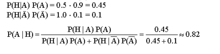
The updated posterior probability P(A|H) = 0.82; then, tossing again, they get heads again (H), and after two heads, the new updated value is P(A|HH) = 0.69; after three heads, the updated value is P(A|HHH) = 0.53. In this way, if they keep tossing and get heads four times in a row, the new updated value is P(A|HHHH) = 0.36. At this point, the observer’s confidence in the fairness of the coin has decreased significantly; starting from a confidence of 0.5, they have already begun to doubt the fairness of the coin. After four consecutive heads, they are more inclined to believe that the coin is likely a fake coin with both sides being heads!

From the above examples, we have a preliminary understanding of Bayes’ theorem and its simple applications.

The Significance of Bayes’ Theorem

Bayes’ theorem is the greatest contribution of Bayes to probability theory and statistics, but at that time, Bayes’ research on “inverse probability” and the derived Bayes’ theorem seemed plain and unremarkable, failing to attract attention, and Bayes remained unknown. Today, this should not be the case at all. The important significance of the Bayes formula is the method of probing unknown probabilities, as illustrated in Example 3. People first have a prior guess, then combine observational data to revise the prior and obtain a more reasonable posterior probability. This means that when you cannot accurately know the essence of a certain thing, you can rely on experience to gradually approach the state of the unknown world, thus judging its essential properties. In fact, its profound ideas far exceed what an average person can recognize; perhaps Bayes himself was not fully aware of this during his lifetime. Due to such an important achievement, he did not publish it during his lifetime; it was only after his death in 1763 that a friend published it. Later, Laplace proved a more general version of Bayes’ theorem and applied it in celestial mechanics and medical statistics. Today, Bayes’ theorem is a foundational framework commonly used in machine learning in contemporary artificial intelligence.【3】.

Bayes’ theorem contradicts classical statistics of the time and even seems somewhat “unscientific”. Therefore, it has been buried for many years and not favored by scientists. As seen in the previous section, Example 3 shows that the application method of Bayes’ theorem is based on subjective judgment; one first subjectively guesses a value and then continuously revises it based on empirical facts to finally obtain the essence of the objective world. In fact, this is precisely the scientific method, as well as the way humans recognize the world (learn) from childhood. Therefore, it can be said that one of the key factors in the flourishing development of artificial intelligence research in recent years is the “marriage” of classical computing technology and probability statistics. Among them, the Bayes formula summarizes the principles of the learning process of humans, and when combined with big data training, it is possible to more accurately simulate the human brain, teaching machines to “learn”, thereby accelerating the progress of AI. Current circumstances indeed reflect this.

How Do Machines Learn?

What do we teach machines to learn? In fact, it is about learning how to process data, which is also what adults teach children: to mine useful information from the vast amounts of data obtained from the senses. If we describe this in mathematical terms, it means to model from data and abstract the parameters of the model【4】.

The tasks of machine learning include major functions such as “regression” and “classification”. Regression is a commonly used method in statistics, aimed at solving the parameters of a model to “regress” things to their original state. Classification is also an important part of machine learning. Categorizing things is the first step in human cognition of the world from infancy. Mothers teach children: this is a dog, that is a cat. This learning method belongs to “supervised” learning, guided by the mother. Learning can also be “unsupervised”; for example, children see “birds flying in the sky, planes, etc.,” and “fish swimming in the water, submarines, etc.,” and can naturally categorize these things into two broad categories: “flying objects” and “swimming objects”.

Bayes’ formula can also be used to classify data. Let’s illustrate with an example.

Suppose we have tested data from 1000 fruits, including the following three characteristics: shape (long?), taste (sweet?), color (yellow?), and these fruits include three types: apples, bananas, or pears, as shown in Figure 2. Now, using a Bayesian classifier, how will it determine the category of a newly given fruit? For example, if this fruit has all three characteristics: long, sweet, and yellow, then the Bayesian classifier should be able to provide the probability of this new fruit being each type of fruit based on the known training data.

First, let’s see what we can get from the data of 1000 fruits.

1. Among these fruits, 50% are bananas, 30% are apples, and 20% are pears.That is, P(banana) = 0.5, P(apple) = 0.3, P(pear) = 0.2.

2. Among 500 bananas, 400 (80%) are long, 350 (70%) are sweet, and 450 (90%) are yellow.That is, P(long|banana) = 0.8, P(sweet|banana) = 0.7, P(yellow|banana) = 0.9.

3. Among 300 apples, 0 (0%) are long, 150 (50%) are sweet, and 300 (100%) are yellow.That is, P(long|apple) = 0, P(sweet|apple) = 0.5, P(yellow|apple) = 1.

4. Among 200 pears, 100 (50%) are long, 150 (75%) are sweet, and 50 (25%) are yellow.That is, P(long|pear) = 0.5, P(sweet|pear) = 0.75, P(yellow|pear) = 0.25.

In the above description, P(A|B) indicates the probability of A occurring when condition B is met. For example, P(sweet|pear) indicates the probability of pears being sweet, and P(pear|sweet) indicates the probability of pears appearing among sweet fruits.

Figure 2: Bayesian Classifier

The so-called “naive Bayesian classifier” uses the term “naive” to indicate that the information expressed in the data is independent of each other. In this specific case, it means that the three characteristics of the fruit, “long, sweet, yellow,” are independent of each other, as they describe the shape, taste, and color of the fruit, which are unrelated. The term “Bayesian” indicates that this type of classifier utilizes Bayes’ formula to calculate posterior probabilities, i.e., P(A|new data) = P(new data|A) P(A)/ P(new data).

Here, “new data” = “long sweet yellow”. Next, we will calculate the probabilities that this fruit is a banana, apple, or pear under the condition of “long sweet yellow”. For bananas:

P(banana|long sweet yellow) = P(long sweet yellow|banana) P(banana)/ P(long sweet yellow)

The first term on the right:P(long sweet yellow|banana) = P(long|banana) * P(sweet|banana) * P(yellow|banana) = 0.8*0.7*0.9 = 0.504.

In the above calculation, P(long sweet yellow|banana) is expressed as the product of three probabilities because of the independence of the features.

Finally, we find: P(banana|long sweet yellow) = 0.504*0.5/ P(long sweet yellow) = 0.252/ P(long sweet yellow).

A similar method is used to calculate the probability for apples:P(long sweet yellow|apple) = P(long|apple)*P(sweet|apple) * P(yellow|apple) = 0*0.5*1 = 0.P(apple|long sweet yellow) = 0.

Denominator: P(long sweet yellow) = P(long sweet yellow|banana) P(banana) + P(long sweet yellow|apple) P(apple) + P(long sweet yellow|pear) P(pear)= 0.27073

Finally, we get: P(banana|long sweet yellow) = 93%

P(apple|long sweet yellow) = 0

P(pear|long sweet yellow) = 7%

Therefore, when you give me a fruit that is long, sweet, and yellow, the conclusion drawn by the Bayesian classifier trained on 1000 fruits is that this new fruit is unlikely to be an apple (0% probability), has a very small chance (7%) of being a pear, and has the greatest likelihood (93%) of being a banana.

The Secrets of Deep Learning

Now, let’s take a look at how children learn to recognize dogs and cats. They do this by being exposed to various dogs and cats by their mothers, and through repeated experiences, they learn the multiple features of dogs and cats, forming their own judgment methods to categorize them into “cats” and “dogs”. Scientists also teach machines to learn in a similar way. For instance, they might distinguish cats from dogs by their ears: “dogs have long ears, cats have short ears,” and “cat ears point up, dog ears point down.” Based on these features, the data can be plotted in a two-dimensional graph, as shown in Figure 3b. At this point, it may be possible to draw a line AB in Figure 3b to easily separate cats and dogs using these two features. Of course, this is just a simple explanation of the “features” and may not truly distinguish between cats and dogs.

Figure 3: Machine Classification

In summary, machines can classify regions based on a certain “feature”. So, where should this line be drawn? This is the problem that the “training” process needs to solve. In machine models, there are parameters known as “weights” w1, w2, w3, …; the process of “training” is to adjust these parameters so that this line AB is drawn in the correct position, pointing in the correct direction. In the aforementioned “cat and dog” example, the output could be 0 or 1, representing cat and dog, respectively. In other words, “training” is like a mother teaching a child to recognize cats and dogs; for the AI model, it involves inputting a large number of labeled photos of cats and dogs, and the AI model adjusts the weight parameters to ensure the output matches the known answers.

Once the trained AI model is completed, it can be used to recognize cat and dog photos without labeled answers. For example, in the example described above: if the data falls on the left side of line AB, output “dog”; if on the right side, output “cat”.

Figure 3b illustrates a very simple case; in most scenarios, a single line cannot distinctly separate two types, as shown in Figures 4a, 4b, and 4c, which depict increasingly complex situations that we will not discuss further.

Figure 4: More Features Require More Parameters for Recognition

Discriminative and Generative Models

In supervised learning models in machine learning, there are two types: discriminative models and generative models. From the previous discussion, we understand how machines “classify”. Based on the names of these two learning methods, we can simply understand that the discriminative model focuses more on classification problems, while the generative model aims to produce samples that meet certain requirements.

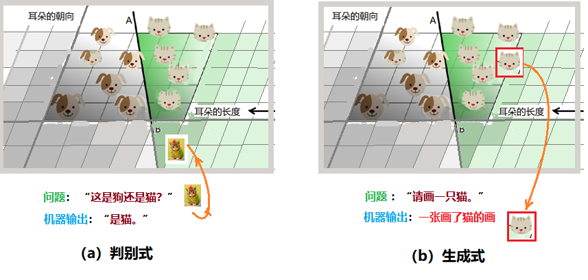
Figure 5: Differences Between Discriminative and Generative Models

Using the example of recognizing “cats and dogs” to illustrate: after showing the child many samples of cats and dogs, if the mother points to a cat and asks the child, “What is this?” The child recalls and responds, “It’s a cat,” which is the discriminative model. If the child answers correctly, they are happy and draw a picture of a cat in their mind, which is the generative model. The machine’s work is similar; as shown in Figure 5, the discriminative model seeks the boundary needed for discrimination to distinguish different types of data instances; the generative model can distinguish between dogs and cats and ultimately draw a “new” animal photo: either a dog or a cat.

In probabilistic terms: let variable Y represent the category and X represent the observable features. The discriminative model has the machine learn the conditional probability distribution P(Y|X), i.e., the probability of category Y given the features X; in the generative model, the machine establishes a joint probability model P(X,Y) for each “category”, thus generating samples that look like a certain type.

For example, if the category Y is “cat, dog” (0,1) and the feature X is the ears’ “up, down” (1,2), suppose we only have four photos as shown:(x,y)= {(1,1),(1,0),(2,0),(2,0)}

Figure 6: Differences in Modeling Between Discriminative and Generative

The discriminative model is built using conditional probability P(Y|X) to obtain the boundary line (the red dashed line in the lower left image); the generative model models the joint probability P(X,Y) for each category, without a boundary line, but delineates the positional intervals of each type in data space (the red circles in the lower right image). The two methods work based on different models’ probabilities. The discriminative model is simpler, focusing only on the boundary line; the generative model needs to model each category and then calculate the posterior probabilities of samples belonging to each category using Bayes’ formula. The generative model is rich in information and flexible but involves complex learning and calculation processes, requiring a large computational burden; if only classification is needed, it is a waste of computational resources.

In recent years, discriminative models have been more favored because they solve problems in a more direct manner and have already been applied in various scenarios, such as classifying spam and normal emails. The 2016 AlphaGo was also a typical example of applying discriminative models for decision-making.

Features of ChatGPT

If you have chatted with ChatGPT, you will be amazed at its wide-ranging capabilities: creating poetry, generating code, drawing, writing papers, seemingly excelling in everything. What gives it such powerful abilities?

From the name ChatGPT, we know it is a “Generative Pre-trained Transformer” (GPT). This includes three meanings: “Generative”, “Pre-trained”, and “Transformer”. The first term clarifies that it uses the generative modeling method introduced above. Pre-trained means it has undergone multiple training phases. The transformer refers to the English translation of “transformer”. The transformer was introduced by a team from Google Brain in 2017 and can be applied to tasks such as translation and text summarization, and is now considered the preferred model for handling natural language processing (NLP) problems with sequential input data.

If you ask ChatGPT about itself, it generally states that it is a large AI language model, referring to the transformer.

This type of language model, in simple terms, is a machine that can perform “word chaining”: input a piece of text, and the transformer outputs a “word” to reasonably continue the input text. (Note: Here, I refer to output as a “word”, but in reality, it is a “token”, which may have different meanings in different languages; in Chinese, it could be a “character”, while in English, it could be a “root word”.)

In fact, language itself is just a form of “word chaining”. Let’s think about how children learn language and writing. They learn to speak a sentence after hearing adults say various sentences many times. Learning to write is similar; people say, “Reading 300 Tang poems, even if you can’t write poetry, you can recite it.” When students read a lot of others’ articles and begin to learn writing, they will inevitably imitate, essentially unconsciously learning “word chaining”.

Figure 7: Language Model

Therefore, in reality, the task of a language model seems very simple; it basically keeps asking, “What should the next word of the input text be?” As shown in Figure 7, after the model selects an output word, this word is added to the original text, which then serves as input again for the language model, asking the same question, “What is the next word?” Then, it outputs, adds to the text, inputs, selects… and so on until a “reasonable” text is generated.

The “reasonableness” of the text generated by the machine model depends heavily on the quality of the “generative model” used, as well as the level of “pre-training”. Internally, for a given input text, the model produces a ranking list of possible words that could follow, along with the corresponding probabilities for each word. For example, if the input is “spring breeze”, the next possible “character” could be many; let’s list just 5 for now: “blow 0.11, warm 0.13, again 0.05, to 0.1, dance 0.08,” etc., with each number representing the probability of its occurrence. In other words, the model provides a long list of words with probabilities. So, which one should be chosen?

If we always choose the one with the highest probability, it probably wouldn’t be “reasonable.” Let’s think again about the process of students learning to write. Although it is also a form of “word chaining,” different people and different times have various ways of chaining words. This is how diverse and creative articles can be written. Therefore, the machine should also be given random opportunities to choose from different probabilities to avoid monotony and produce colorful and interesting works. Although it is not advisable to always choose the highest probability, it is best to select one with a relatively high probability to create a “reasonable model.”

ChatGPT is a large language model, and this “large” is primarily reflected in the number of parameters in the model’s neural network. The number of parameters is a key factor determining its performance. These parameters need to be set before training and can control the grammar, semantics, and style of the generated language, as well as the behavior of language understanding. They can also control the behavior of the training process and the quality of the generated language.

OpenAI’s GPT-3 model has 175 billion parameters, and ChatGPT is considered to be GPT-3.5, with a parameter count likely exceeding 175 billion. These parameters refer to the values that need to be predetermined before training the model. In practical applications, it is often necessary to determine the appropriate number of parameters through experimentation to achieve optimal performance.

These parameters are adjusted through thousands of training processes to yield a good neural network model. It is said that the training cost for GPT-3 was $4.6 million, with a total training cost of $12 million.

As mentioned above, the specialty of ChatGPT is generating text that is “similar to human works.” However, something that can generate grammatically correct language may not necessarily perform well in mathematical calculations, logical reasoning, and other types of tasks, because the expressions in these fields are entirely different from natural language text. This explains why it often fails in mathematical tests.

Additionally, people often find humorous anecdotes about ChatGPT “seriously talking nonsense.” The reason is not hard to understand, primarily related to training biases. If it encounters something it has never heard of, it certainly cannot provide a correct answer. The issues arising from polysemy also confuse the machine model. For example, it is said that when someone asked ChatGPT, “What is the tuning method for the string instrument called ‘gou san gu xian wu’ in ancient China,” it seriously answered, “This is a tuning method for a kind of musical instrument called ‘qin’, and then fabricated a lot of information, which was quite amusing.

In summary, ChatGPT has achieved success right from the start, a strong start, which is also a victory for probability theory and a victory for Bayes.

References

1.Tianrong Zhang. Talking About Probability–From Dice Rolling to AlphaGo[M].Beijing:Tsinghua University Press,pp.71-75,2017.

2.Sean R Eddy,“What is Bayesian statistics?”,[J], Nature Biotechnology 22, 1177 – 1178 (2004) .

3.Jake VanderPlas,“Frequentism and Bayesianism: A Python-driven Primer”,[L], arXiv:1411.5018 [astro-ph.IM],2014. https://arxiv.org/abs/1411.5018

4.Russell, Stuart; Norvig, Peter (2003) [1995]. Artificial Intelligence: A Modern Approach (2nd ed.).[M], Prentice Hall. p.90