Click the card below to follow the “CVer” WeChat public account
AI/CV heavy content delivered instantly
Click to join —> the CV WeChat technical exchange group
Reprinted from: New Intelligence | Edited by: Xinpeng Hao Kun
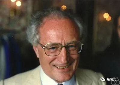
[Guide] Recently, Jürgen Schmidhuber, the father of LSTM, reviewed the history of artificial intelligence since the 17th century. In this lengthy article, Schmidhuber provides readers with a timeline of significant events in the fields of neural networks, deep learning, and artificial intelligence, as well as the scientists who laid the foundations for AI.
Annotated History of Modern AI and Deep Learning
https://people.idsia.ch/~juergen/deep-learning-history.html
Paper: https://arxiv.org/abs/2212.11279
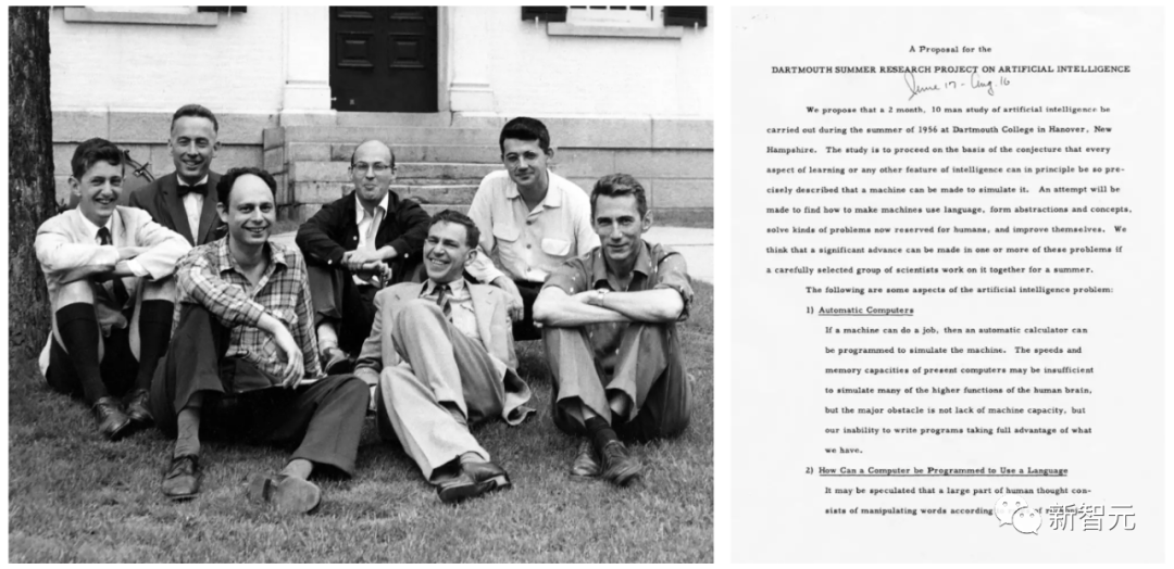
The term “artificial intelligence” was first officially proposed at the Dartmouth Conference in 1956 by John McCarthy and others.
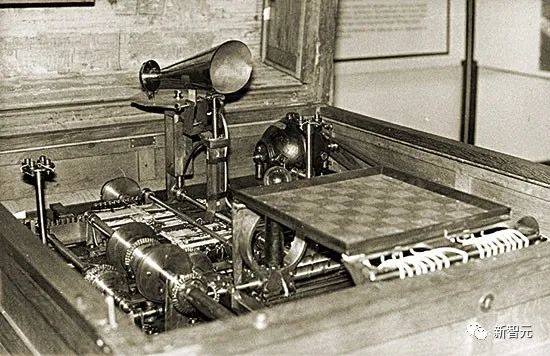
The proposal of practical AI can be traced back to 1914 when Leonardo Torres y Quevedo built the first working chess machine terminal game player. At that time, chess was considered an activity limited to intelligent biological beings.
As for the theory of artificial intelligence, it can be traced back to 1931-34. At that time, Kurt Gödel established fundamental limitations of any type of computational-based artificial intelligence.
Fast forward to the 1980s, the history of AI at that time emphasized topics like theorem proving, logic programming, expert systems, and heuristic search.
The early 2000s history of AI emphasized topics such as support vector machines and kernel methods. Bayesian reasoning and other probabilistic and statistical concepts, decision trees, ensemble methods, swarm intelligence, and evolutionary computation drove many successful AI applications.
AI research in the 2020s has become more “retro”, emphasizing concepts such as the chain rule and deep nonlinear artificial neural networks trained through gradient descent, particularly feedback-based recurrent networks.
Schmidhuber states that this article corrects the previously misleading “history of deep learning”. He believes that previous histories of deep learning overlooked most of the pioneering work mentioned in the article.
Additionally, Schmidhuber refuted a common misconception that neural networks “were introduced in the 1980s as tools to help computers recognize patterns and simulate human intelligence”. In fact, neural networks appeared long before the 1980s.
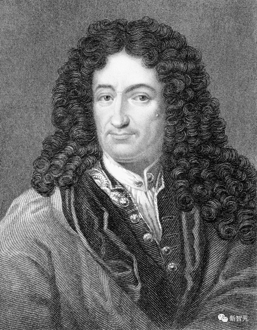
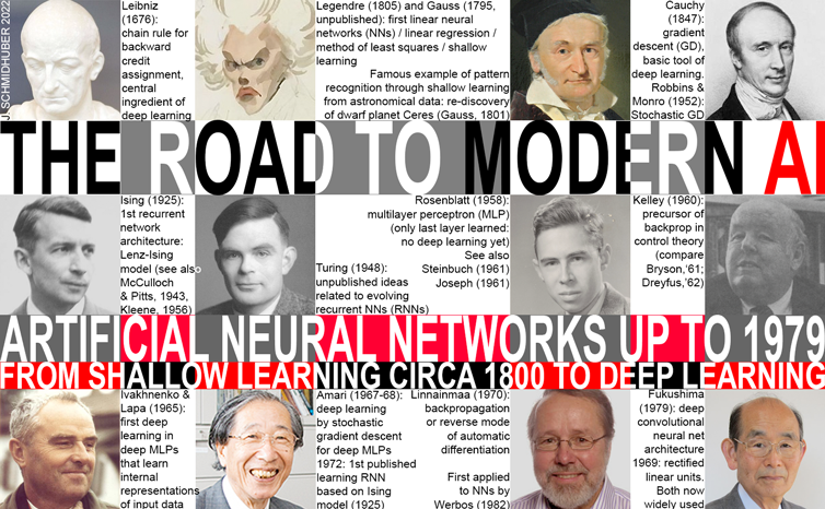
1. 1676: The Chain Rule of Backpropagation
In 1676, Gottfried Wilhelm Leibniz published the chain rule of calculus in his memoirs. Today, this rule has become central to credit assignment in deep neural networks and is foundational to modern deep learning.
Gottfried Wilhelm Leibniz
Neural networks consist of nodes or neurons that compute differentiable functions of inputs from other neurons, which in turn compute differentiable functions of inputs from other neurons. To understand how changes to the parameters or weights of earlier functions affect the final function output, the chain rule is necessary.
This answer is also used in gradient descent techniques. To train the neural network to convert input patterns from the training set into desired output patterns, all neural network weights are iteratively adjusted slightly in the direction of maximum local improvement, creating a slightly better neural network, and so on, gradually approaching the optimal combination of weights and biases to minimize the loss function.
Notably, Leibniz was also the first mathematician to discover calculus. He and Isaac Newton independently discovered calculus, and the mathematical notation he used has been more widely adopted; Leibniz’s notation is generally considered more comprehensive and broadly applicable.
Moreover, Leibniz is also known as “the world’s first computer scientist”. He designed the first machine capable of performing all four arithmetic operations in 1673, laying the foundation for modern computer science.
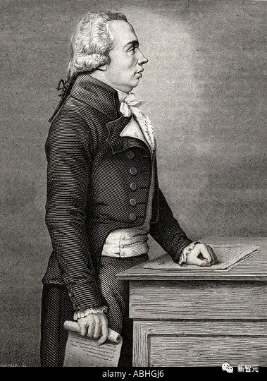
2. Early 19th Century: Neural Networks, Linear Regression, and Shallow Learning
In 1805, Adrien-Marie Legendre published content that is now commonly referred to as linear neural networks.
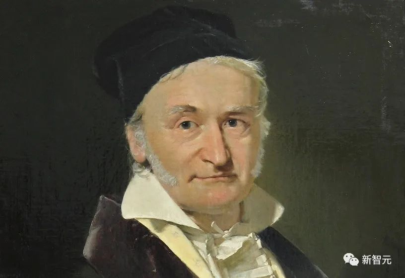
Later, Johann Carl Friedrich Gauss was also recognized for similar research.
This neural network from over two centuries ago has two layers: an input layer with multiple input units and an output layer. Each input unit can store a real number and is connected to the output through connections with real-valued weights.
The output of the neural network is the sum of the products of the inputs and their weights. Given a training set of input vectors and the expected target value for each vector, the weights are adjusted to minimize the sum of the squared differences between the neural network output and the corresponding targets.
Of course, it wasn’t called a neural network back then. It was known as the least squares method, also widely referred to as linear regression. However, mathematically, it is the same as today’s linear neural networks: the same fundamental algorithm, the same error function, the same adaptive parameters/weights.
Johann Carl Friedrich Gauss
This simple neural network performs “shallow learning”, in contrast to “deep learning” with many nonlinear layers. In fact, many neural network courses start by introducing this method before moving on to more complex, deeper networks.
Today, all students in technical disciplines must take mathematics courses, especially in analysis, linear algebra, and statistics. Many important results and methods in all these fields can be attributed to Gauss: the fundamental theorem of algebra, Gaussian elimination, and the Gaussian distribution in statistics, among others.
This person, who is said to be “the greatest mathematician of all time”, also pioneered differential geometry, number theory (his favorite subject), and non-Euclidean geometry. Without his contributions, modern engineering, including AI, would be unimaginable.
3. 1920-1925: The First Recurrent Neural Network
Similar to the human brain, recurrent neural networks (RNNs) have feedback connections, allowing them to follow directed connections from some internal nodes to others and ultimately return to the starting point. This is crucial for remembering past events during sequence processing.
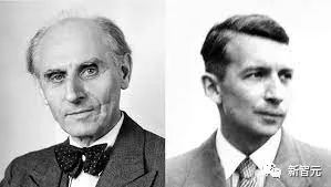
William Lenz (left); Ernst Ising (right)
Physicists Ernst Ising and Wilhelm Lenz introduced and analyzed the first non-learning RNN architecture in the 1920s: the Ising model. It enters a balanced state based on input conditions and is the basis for the first learning model of RNNs.
In 1972, Shun-Ichi Amari made the Ising model’s recurrent architecture adaptive, allowing it to learn associations between input patterns and output patterns by changing its connection weights. This was the world’s first learning RNN.
Currently, the most popular RNN is the Long Short-Term Memory (LSTM) network proposed by Schmidhuber. It has become the most cited neural network of the 20th century.
4. 1958: Multi-Layer Feedforward Neural Networks
In 1958, Frank Rosenblatt combined linear neural networks with threshold functions to design a deeper multi-layer perceptron (MLP).
The multi-layer perceptron follows the principles of the human nervous system, learning and making data predictions. It first learns, then uses weights to store data, and employs algorithms to adjust weights and reduce bias during training, i.e., the error between actual values and predicted values.
Due to the frequent use of backpropagation algorithms for training multi-layer feedforward networks, it has become a standard supervised learning algorithm in the field of pattern recognition and continues to be a subject of research in computational neuroscience and parallel distributed processing.
5. 1965: The First Deep Learning
The successful learning of deep feedforward network architectures began in 1965 in Ukraine, when Alexey Ivakhnenko and Valentin Lapa introduced the first universal working learning algorithm for deep MLPs with an arbitrary number of hidden layers.
Given a training set of input vectors with corresponding target output vectors, the layers gradually increase and are trained through regression analysis, followed by pruning with a separate validation set, where regularization is used to eliminate redundant units. The number of layers and the units in each layer learn in a problem-relevant manner.
Like later deep neural networks, Ivakhnenko’s networks learned to create hierarchical, distributed, internal representations for incoming data.
He did not call them deep learning neural networks, but that is what they were. In fact, the term “deep learning” was first introduced to machine learning by Dechter in 1986, and the concept of “neural networks” was introduced by Aizenberg et al. in 2000.
6. 1967-68: Stochastic Gradient Descent
In 1967, Shun-Ichi Amari first proposed training neural networks through stochastic gradient descent (SGD).
Amari and his student Saito learned internal representations in a five-layer MLP with two modifiable layers, which were trained to classify non-linearly separable pattern classes.
Rumelhart, Hinton, and others did similar work in 1986, naming it the backpropagation algorithm.
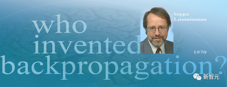
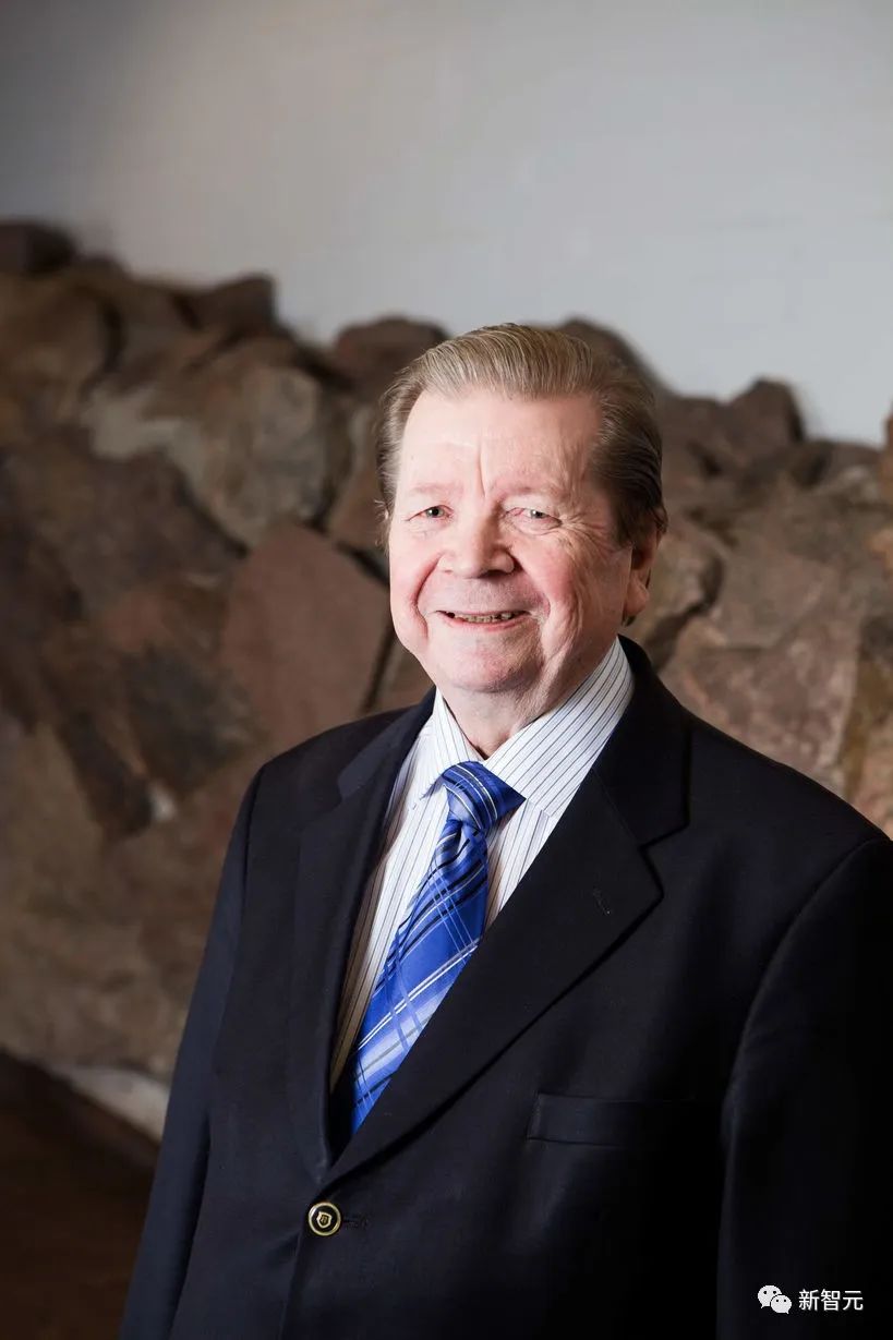
7. 1970: The Backpropagation Algorithm
In 1970, Seppo Linnainmaa first published the backpropagation algorithm, a famous credit assignment algorithm for differentiable node networks, also known as “reverse mode of automatic differentiation”.
Linnainmaa first described an efficient way of error backpropagation for class neural networks in arbitrary, discrete, sparse connections. It is now the basis for widely used neural network software packages, such as PyTorch and Google’s TensorFlow.
Backpropagation is essentially an efficient way to implement Leibniz’s chain rule for deep networks. The gradient descent proposed by Cauchy gradually weakens certain neural network connections while strengthening others during many experimental processes.
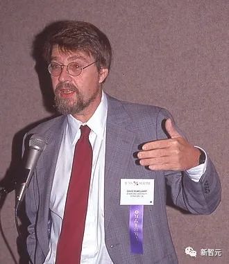
By 1985, computational costs had decreased by about 1,000 times compared to 1970, when desktop computers were just becoming common in wealthy academic labs, and David Rumelhart and others conducted experimental analyses of known methods.
Through experiments, Rumelhart and others demonstrated that backpropagation could generate useful internal representations in the hidden layers of neural networks. At least for supervised learning, backpropagation is typically more effective than the deep learning conducted by Amari through the SGD method mentioned above.
Before 2010, many believed that training multi-layer neural networks required unsupervised pre-training. In 2010, Schmidhuber’s team, along with Dan Ciresan, showed that deep FNNs could be trained through simple backpropagation without needing unsupervised pre-training for important applications.
8. 1979: The First Convolutional Neural Network
In 1979, Kunihiko Fukushima developed a neural network model for pattern recognition at STRL: the Neocognitron.
However, this Neocognitron, in today’s terms, is called a convolutional neural network (CNN), which is one of the greatest inventions of the fundamental structure of deep neural networks and is a core technology of current artificial intelligence.
The Neocognitron introduced by Dr. Fukushima was the first neural network to use convolution and down-sampling and is the prototype of convolutional neural networks.
Dr. Fukushima designed an artificial multi-layer neural network with learning capabilities that could mimic the brain’s visual network, and this “insight” became the foundation of modern AI technology. Dr. Fukushima’s work has led to a series of practical applications, from self-driving cars to facial recognition, from cancer detection to flood prediction, with even more applications to come.
In 1987, Alex Waibel combined convolutional neural networks with weight sharing and backpropagation to propose the concept of time-delay neural networks (TDNN).
Since 1989, Yann LeCun’s team has contributed to the improvement of CNNs, especially in terms of images.
By the end of 2011, Schmidhuber’s team greatly accelerated the training speed of deep CNNs, making them more popular in the machine learning community. The team launched the GPU-based CNN: DanNet, which was deeper and faster than earlier CNNs. That same year, DanNet became the first pure deep CNN to win a computer vision competition.
The residual neural network (ResNet) proposed by four scholars from Microsoft Research won first place in the 2015 ImageNet Large Scale Visual Recognition Challenge.
Schmidhuber stated that ResNet is an early version of the fast neural networks (Highway Net) developed by his team. Compared to previous neural networks, which had at most a few dozen layers, this was the first truly effective deep feedforward neural network with hundreds of layers.
9. 1987-1990: Graph Neural Networks and the Random Delta Rule
Deep learning architectures capable of manipulating structured data (e.g., graphs) were proposed by Pollack in 1987 and expanded upon and improved by Sperduti, Goller, and Küchler in the early 1990s. Today, graph neural networks are used in many applications.
Paul Werbos and R. J. Williams analyzed methods for implementing gradient descent in RNNs. Teuvo Kohonen’s self-organizing maps also gained popularity.
In 1990, Stephen Hanson introduced the random delta rule, a stochastic method for training neural networks through backpropagation. Decades later, this method became popular under the nickname “dropout”.
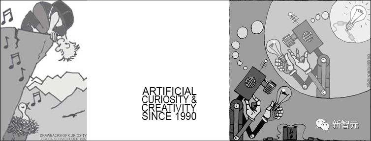
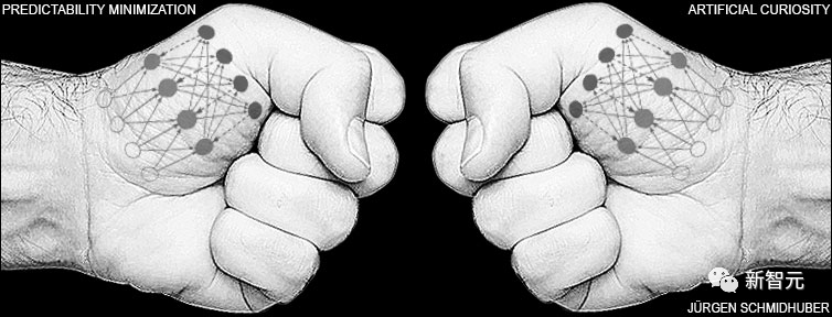
10. February 1990: Generative Adversarial Networks / Curiosity
Generative Adversarial Networks (GANs) were first published in 1990 under the title “Artificial Intelligence Curiosity”.
Two opposing neural networks (one probabilistic generator and one predictor) attempt to maximize each other’s loss in a minimax game. Among them:
-
The generator (called the controller) generates probabilistic outputs (using random units, such as later StyleGAN).
-
The predictor (called the world model) sees the controller’s output and predicts the environment’s response to them. Using gradient descent, the predictor NN minimizes its error, while the generator NN tries to maximize this error—one network’s loss is the other’s gain.
Four years before the paper on GANs was published in 2014, Schmidhuber summarized the 1990 generative adversarial NN in a famous 2010 survey: “A neural network used to maximize the intrinsic reward of a controller is used to predict the world model, proportional to the model’s prediction error.”
The subsequently released GANs are just an instance. The experiments were very short, and the environment returned 1 or 0 based on whether the controller’s (or generator’s) output was within a given set.
The principles of 1990 have been widely used in reinforcement learning exploration and the synthesis of realistic images, although the latter’s domain has recently been replaced by Rombach et al.’s Latent Diffusion.
In 1991, Schmidhuber published another ML method based on two adversarial NNs called predictability minimization, used to create separable representations of partially redundant data, applied in images in 1996.
11. April 1990: Generating Subgoals / Working by Instructions
For centuries, most NNs have focused on simple pattern recognition rather than advanced reasoning.
However, in the early 1990s, exceptions began to emerge. This work injected the concept of traditional “symbolic” hierarchical artificial intelligence into end-to-end differentiable “sub-symbolic” NNs.
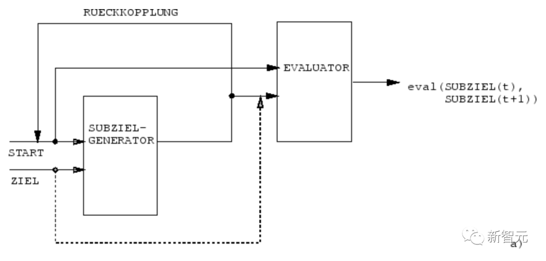
In 1990, Schmidhuber’s team of NNs learned to generate hierarchical action plans using a subgoal generator of end-to-end differentiable NNs for hierarchical reinforcement learning (HRL).
A reinforcement learning machine receives additional command input in the form of (start, goal). An evaluator NN learns to predict the current reward/cost from start to goal. A subgoal generator based on (R)NN also sees (start, goal) and learns a series of intermediate subgoals with the lowest cost using the evaluator NN’s (copy) through gradient descent. The RL machine attempts to achieve the final goal using this sequence of subgoals.
This system learns action plans at multiple levels of abstraction and multiple time scales and, in principle, addresses what has recently been referred to as the “open-ended problem”.
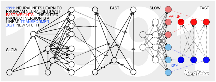
12. March 1991: Transformers with Linear Self-Attention
Transformers with “linear self-attention” were first published in March 1991.
These so-called “Fast Weight Programmers” or “Fast Weight Controllers” separate storage and control like traditional computers but in an end-to-end differentiable, adaptive, and neural network manner.
Moreover, today’s Transformers extensively use unsupervised pre-training, a deep learning method first published by Schmidhuber in 1990-1991.
13. April 1991: Distilling One NN into Another
Using the NN distillation procedure proposed by Schmidhuber in 1991, the hierarchical internal representations of the aforementioned neural historical compressor can be distilled into a single recursive NN (RNN).
Here, the knowledge of the teacher NN is “distilled” into the student NN by training the student NN to imitate the behavior of the teacher NN (while also retraining the student NN to ensure that previously learned skills are not forgotten). The NN distillation method was also republished many years later and is widely used today.
14. June 1991: The Fundamental Problem — Gradient Vanishing
Sepp Hochreiter, Schmidhuber’s first student, discovered and analyzed the fundamental deep learning problem in his graduation thesis in 1991.
Deep NNs are plagued by the now-famous gradient vanishing problem: in typical deep or recurrent networks, the error signals in backpropagation either shrink rapidly or grow beyond limits. In both cases, learning fails.
15. June 1991: Foundations of LSTM/Highway Net/ResNet
Long Short-Term Memory (LSTM) recurrent neural networks overcome the fundamental deep learning problems identified by Sepp Hochreiter in the aforementioned 1991 graduation thesis.
After the publication of the peer-reviewed paper in 1997 (now the most cited NN paper of the 20th century), Schmidhuber’s students Felix Gers and Alex Graves further improved LSTM and its training procedures.
The LSTM variant with a forget gate, published in 1999-2000, is still applied in Google’s TensorFlow today.
In 2005, Schmidhuber first published articles on LSTM’s complete backpropagation in time and bidirectional propagation (also widely used).
A milestone training method in 2006 was “Connectionist Temporal Classification” (CTC), used for aligning and recognizing sequences simultaneously.
In 2007, Schmidhuber’s team successfully applied CTC-trained LSTM to speech (also with hierarchical LSTM stacks), achieving exceptional end-to-end neural speech recognition results for the first time.
In 2009, through Alex’s efforts, CTC-trained LSTM became the first RNN to win international competitions, specifically three ICDAR 2009 handwriting contests (French, Persian, Arabic). This sparked significant interest in the industry. LSTM was soon applied in all scenarios involving sequential data, such as speech and video.
In 2015, the combination of CTC and LSTM greatly improved voice recognition performance on Google Android smartphones. Until 2019, Google’s voice recognition on mobile devices was still based on LSTM.
1995: Neural Probabilistic Language Models
In 1995, Schmidhuber proposed an excellent neural probabilistic text model, the basic concept of which was reused in 2003.
In 2001, Schmidhuber showed that LSTM could learn languages that traditional models like HMM could not learn.
Google Translate in 2016 was based on two interconnected LSTMs (the white paper mentioned LSTM over 50 times), one for incoming text and one for outgoing translations.
That same year, over a quarter of Google’s supercomputing power used for inference was dedicated to LSTM (with another 5% allocated to another popular deep learning technique, CNN).
By 2017, LSTM also supported Facebook’s machine translation (over 30 billion translations weekly), Apple’s Quicktype on about 1 billion iPhones, Amazon’s Alexa voice, Google’s image captioning generation, and automatic email responses.
Of course, Schmidhuber’s LSTM has also been widely used in healthcare and medical diagnostics—an easy Google Scholar search can find countless medical articles with “LSTM” in their titles.
In May 2015, Schmidhuber’s team proposed the Highway Network based on LSTM principles, the first very deep FNN with hundreds of layers (previous NNs had at most a few dozen layers). Microsoft’s ResNet (which won the ImageNet 2015 competition) is a version of it.
The early Highway Net performed similarly to ResNet on ImageNet. Variants of Highway Net have also been used in certain algorithmic tasks where pure residual layers do not perform well.
The Principles of LSTM/Highway Net are Core to Modern Deep Learning
The core of deep learning is the depth of NNs.
In the 1990s, LSTM brought fundamentally unlimited depth to supervised recurrent NNs; in 2000, Highway Net, inspired by LSTM, brought depth to feedforward NNs.
Today, LSTM has become the most cited NN of the 20th century, while one of the versions of Highway Net, ResNet, is the most cited NN of the 21st century.
18. 1980 to Present: Learning Actions in NNs Without Teachers
Moreover, NNs are related to reinforcement learning (RL).
While some problems can be solved by non-neural techniques invented as early as the 1980s, such as Monte Carlo tree search (MC), dynamic programming (DP), artificial evolution, α-β pruning, control theory, and system identification, stochastic gradient descent, and general search techniques, deep FNNs and RNNs can offer better performance for certain types of RL tasks.
In general, reinforcement learning agents must learn how to interact with a dynamic, initially unknown, partially observable environment without help from teachers, maximizing the expected cumulative reward signal. There may be arbitrary, prior unknown delays between actions and perceivable outcomes.
When the environment has a Markov interface that allows the RL agent’s input to convey all information needed to determine the next best action, RL based on dynamic programming (DP)/temporal difference (TD)/Monte Carlo tree search (MC) can be very successful.
In more complex situations without a Markov interface, the agent must consider not only the current input but also the history of previous inputs. In this regard, the combination of RL algorithms and LSTM has become a standard solution, particularly LSTM trained through policy gradients.
For example, in 2018, an LSTM trained by PG was at the core of OpenAI’s famous Dactyl, which learned to control a dexterous robotic hand without a teacher.
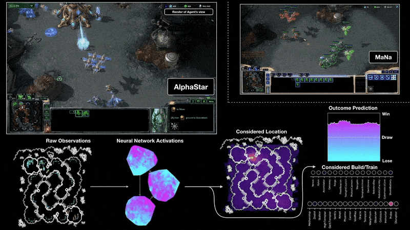
In 2019, DeepMind (co-founded by a student from Schmidhuber’s lab) defeated professional players in the game StarCraft, using Alphastar, which had a deep LSTM core trained by PG.
Meanwhile, the RL LSTM (which accounted for 84% of the total model parameters) was also at the core of the famous OpenAI Five, which defeated professional human players in Dota 2.
The future of RL will involve learning/combining/planning actions using compact spatiotemporal abstractions of complex input streams, concerning common-sense reasoning and learning to think.
In his papers published in 1990-91, Schmidhuber proposed a self-supervised neural historical compressor that can learn multi-layered abstractions and representation concepts over multiple time scales; the subgoal generator based on end-to-end differentiable NNs can learn hierarchical action plans through gradient descent.
In the subsequent years of 1997 and 2015-18, methods for learning abstract thinking became more complex and were published.
19. It’s a Hardware Problem, Dummy!
Over the past thousand years, significant breakthroughs in deep learning algorithms would not have been possible without continuously improving and accelerating computer hardware.
The first known gear computing device was the Antikythera mechanism from ancient Greece over 2000 years ago. This is the oldest known complex scientific computer and the first analog computer in the world.
The Antikythera mechanism
The world’s first practical programmable machine was invented by the ancient Greek mechanic Hero in the 1st century AD.
Machines in the 17th century became more flexible, capable of computing answers based on input data.
The first mechanical calculator for simple arithmetic was invented by Wilhelm Schickard in 1623.
In 1673, Leibniz designed the first machine capable of performing all four arithmetic operations and with memory. He also described the principle of a binary computer controlled by perforated cards and proposed the chain rule, which forms an important part of deep learning and modern artificial intelligence.
Around 1800, Joseph Marie Jacquard and others in France manufactured the first programmable loom—the Jacquard loom. This invention played a crucial role in the future development of other programmable machines (e.g., computers).
They inspired Ada Lovelace and her mentor Charles Babbage to invent the precursor to modern electronic computers: Babbage’s Difference Engine.
In 1843, Lovelace published the world’s first computer algorithm.
Babbage’s Difference Engine
In 1914, the Spaniard Leonardo Torres y Quevedo became the first artificial intelligence pioneer of the 20th century, creating the first chess terminal machine player.
Between 1935 and 1941, Konrad Zuse invented the world’s first operational programmable universal computer: the Z3.
Unlike Babbage’s analytical engine, Zuse used Leibniz’s principle of binary computation instead of traditional decimal computation, greatly simplifying the hardware load.
In 1944, Howard Aiken led a team that invented the world’s first large-scale automatic digital computer, the Mark I.
In 1948, Frederic Williams, Tom Kilburn, and Geoff Tootill invented the world’s first electronic stored-program computer: the Small Scale Experimental Machine (SSEM), also known as the “Manchester Baby”.
Replica of the “Manchester Baby”
Since then, computing power has become faster with the help of integrated circuits (ICs). In 1949, Werner Jacobi of Siemens applied for a semiconductor patent for integrated circuits, allowing multiple transistors on a common substrate.
In 1958, Jack Kilby demonstrated integrated circuits with external wires. In 1959, Robert Noyce proposed the monolithic integrated circuit. Since the 1970s, graphics processing units (GPUs) have been used to accelerate computations through parallel processing. Today, GPUs in computers contain billions of transistors.
Where are the physical limits?
According to the Bremermann limit proposed by Hans Joachim Bremermann, a computer weighing 1 kg and occupying 1 liter can perform at most 10^51 operations per second in up to 10^32 different states.
However, the mass of the solar system is only 2×10^30 kg, and this trend is bound to break in a few centuries, as the speed of light severely limits the acquisition of additional mass in other solar systems.
Thus, the physical limits require that future efficient computing hardware must have many densely placed processors in three-dimensional space to minimize total connection costs, essentially forming a deep, sparsely connected three-dimensional RNN.
Schmidhuber speculates that deep learning methods for such RNNs will become increasingly important.
19. The Theory of Artificial Intelligence Since 1931
The core of modern artificial intelligence and deep learning is primarily based on mathematics from the past few centuries: calculus, linear algebra, and statistics.
In the early 1930s, Gödel established modern theoretical computer science. He introduced a universal coding language based on integers that allowed the formalization of any digital computer’s operations in axiomatic form.
At the same time, Gödel constructed a famous formal statement that systematically enumerated all possible theorems from a countable set of axioms through a given computational theorem verifier. Thus, he established the fundamental limitations of algorithmic theorem proving, computation, and any type of computational-based artificial intelligence.
Additionally, in a famous letter to John von Neumann, Gödel identified one of the most famous open problems in computer science: “P=NP?”.
In 1935, Alonzo Church proved that there was no general solution to Hilbert and Ackermann’s decision problem, drawing a conclusion from Gödel’s result. To do this, he used his other universal coding language, called Untyped Lambda Calculus, which forms the basis of the influential programming language LISP.
In 1936, Alan Turing introduced another universal model: the Turing machine, reiterating the above results. That same year, Emil Post published another independent model of computation.
Konrad Zuse not only created the world’s first operational programmable universal computer but also designed the first high-level programming language—Plankalkül. He applied it to chess in 1945 and to theorem proving in 1948.
Much of the early artificial intelligence in the 1940s to 1970s was focused on theorem proving and Gödel-style deductions through expert systems and logic programming.
In 1964, Ray Solomonoff combined Bayesian (essentially Laplace) probabilistic reasoning with theoretical computer science to derive a mathematically optimal (but computationally infeasible) way to predict future data from past observations.
He, along with Andrej Kolmogorov, founded the theory of Kolmogorov complexity or algorithmic information theory (AIT), formalizing the concept of Occam’s razor by calculating the shortest program for the data, thus transcending traditional information theory.
Self-referential Gödel machines’ more general optimality is not limited to asymptotic optimality.
Nevertheless, for various reasons, this mathematically optimal artificial intelligence is not practically feasible. Instead, practical modern AI is based on suboptimal, limited, yet not extremely understood technologies, such as NNs and deep learning being the focus.
But who knows what the history of artificial intelligence will look like in 20 years?
Click to enter —> CV WeChat technical exchange group

CVPR/ECCV 2022 paper and code download

Reply in the background: CVPR2022 to download the CVPR 2022 paper and code open-source paper collection.
Reply in the background: ECCV2022 to download the ECCV 2022 paper and code open-source paper collection.
Reply in the background: Transformer review to download the latest 3 Transformer review PDFs.

The target detection and Transformer exchange group has been established.

Scan the QR code below or add WeChat: CVer222 to add CVer's assistant WeChat, and you can apply to join the CVer-target detection or Transformer WeChat exchange group. Other vertical directions have also been covered: target detection, image segmentation, object tracking, face detection & recognition, OCR, pose estimation, super-resolution, SLAM, medical imaging, Re-ID, GAN, NAS, depth estimation, autonomous driving, lane detection, model pruning & compression, denoising, dehazing, deraining, style transfer, remote sensing images, behavior recognition, video understanding, image fusion, image retrieval, paper submission & communication, PyTorch, TensorFlow, and Transformers, etc.

Be sure to note: research direction + location + school/company + nickname (e.g., target detection or Transformer + Shanghai + SJTU + Kaka). Following this format will allow for faster approval and invitation to the group.

▲ Scan or add WeChat ID: CVer222 to join the exchange group.

CVer academic exchange group (Knowledge Planet) is here! If you want to learn about the latest, fastest, and best CV/DL/ML paper delivery, quality open-source projects, learning tutorials, and practical training materials, feel free to scan the QR code below to join the CVer academic exchange group, which has gathered thousands of people!

▲ Scan to join the group
▲ Click the card above to follow the CVer public account

Sorting is not easy, please like and share.