The Art of Probability: Deriving Diffusion Model Theory

Introduction

About a year ago in the autumn, I heard friends mention that a tool called StableDiffusion, an AIGC image generation tool, was sweeping through the artist community. At that time, I also tried to deploy this project locally and created some wonderful images (doge), and the results were indeed shockingly excellent. However, I had not thought about delving deeper into the knowledge behind this tool until later when I considered thoroughly learning it during my research, but various matters delayed me. Until today, a year later, being idle at home, I calm down, pick up pen and paper, and derive some mathematics to clarify the solid theoretical foundation behind this powerful tool, which might also be a nice pastime.

This article is merely a learning note from the author, with most of the main content derived from the articles of several Zhihu experts:

Explaining the Diffusion Model (1) DDPM Theory Derivation (https://zhuanlan.zhihu.com/p/565901160)

Explaining the Diffusion Model (2) Score-based SDE Theory Derivation (https://zhuanlan.zhihu.com/p/589106222)

How to Understand SDE in Diffusion Models? (https://www.zhihu.com/question/616179189/answer/3230281054)

And Dr. Song Yang’s paper on Score-Based SDE:

https//arxiv.org/abs/2011.13456

And Google Research’s work on the Diffusion Model framework:

https//arxiv.org/abs/2208.11970

Concept Introduction

The diffusion model (Diffusion) is a model based on the Markov process, achieving content generation through a multi-step noise addition/removal process. It is very similar to the VAE we learned before, requiring a three-step process: original image → Gaussian noise → generated image.

Note: From my personal experience, the big picture of these generative models is actually quite similar: they all go through the process of original image → white noise → new image, and mathematically, they are all samplers that sample instances from a certain probability distribution (which will be explained later). The biggest difference of Diffusion compared to previous models is probably the introduction of differential ideas, making the generation process more granular (fine) and controllable.

A certain dalao (https//lilianweng.github.io/posts/2021-07-11-diffusion-models/) created a comparison chart of several generative models as follows:

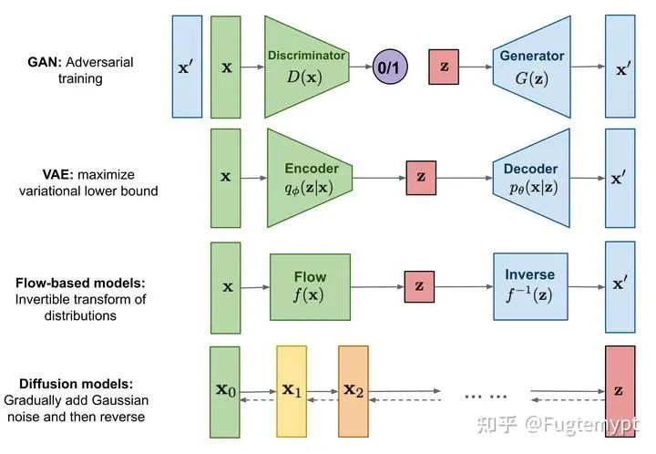
In practice, there are many implementation methods for the Diffusion Model, such as Stable Diffusion based on VAE compression of latent space, or DDPM that does not compress latent space (meaning keeping the latent space size consistent with the original image). This article will not discuss the specific implementation details but will clarify the entire process of Diffusion from a general theoretical perspective. However, if one understands this process thoroughly, it will not be difficult to look at specific implementation methods.

Process Overview

The training process of the Diffusion Model can be roughly divided into two stages: the first stage is the noise addition stage, where given an original image, we will add noise to it step by step, ultimately turning it into Gaussian noise; the second stage is the noise removal stage, where we will attempt to restore the noisy image back to the original image. When inference is performed after training, we do not conduct the first stage, but take a white noise and then perform the second stage, and the image obtained after “restoration” is the image generated by the model.

Note: How does an image relate to a random variable? Assuming the original image is a tensor of size , then the value at each position is a definite number, which seems unrelated to random variables. However, do not forget that we are not training on a single image but on a whole class of images. If we have images of faces (all of size ), then at each position, there are values, which can be viewed as a probability distribution. These probability distributions represent all the features of this class of images; for example, the area near the center of the screen is usually skin-colored, so the variance of the probability distribution here will be small, and the mean of the RGB three channels will combine to produce “skin color”.

The vast majority of Diffusion Models are implemented based on the above process, and their differences usually lie in the methods of “adding noise” and “removing noise”. Of course, it is difficult to derive the content of the model based solely on an abstract framework; here, we attempt to be more specific by deriving some aspects of the popular DDPM (Denoising Diffusion Probabilistic Models (https//arxiv.org/abs/2006.11239)).

Noise Addition Process/Forward Process

Assuming our noise addition process has already gone through steps, now we want to perform an addition of noise. A natural idea is to construct a linear relationship between the image and the noise:

Where

The recursive form is not easy to solve; we consider whether we can write it in a general form:

Let us assume that are independent; based on the additivity of the normal distribution, the above can be written as

Which is a bit ugly because it contains both and , making it difficult to simplify. Can we try to normalize these two parameters, that is, let to eliminate one of the variables? Since we hope to ultimately obtain the image , normalization will not affect our goal, hence we attempt normalization, yielding

Thus we can let , leading to , allowing (3) to be rewritten as

Similarly, with , we can rewrite (1) as

Expressing the above two equations in terms of probability distributions, we have

The entire forward process can be expressed as

Noise Removal Process/Backward Process

In the noise removal process, we aim to achieve the transformation from pure noise to the real image . For this, we also consider each step , but unlike the forward process, we do not model it as a simple linear relationship (but still model it as a normal distribution), allowing the model to learn the expectation and variance of each step of the noise removal process through the parameters of a neural network.

In fact, this looks like learning the reverse distribution of the forward process, which we will mention again later.

Accumulating all steps yields the probability distribution of the entire stochastic process

Note: This is the probability distribution of the entire stochastic process , not the distribution of . To find the distribution of , we need to enumerate all possible and sum (integrate) their corresponding stochastic processes’ probabilities, which is known as the total probability formula.

From the perspective of probability theory, the computation result of our model should be the distribution of (which is the result after the above integration), and our optimization goal is to make as close as possible to the true distribution of , for example, faces. However, we do not know the true distribution of the data , but we have several samples drawn from the true distribution of , so we naturally hope that these samples can have a high probability in the distribution we model (for example, if we have many face images, but the model ends up creating a panda face distribution, then the probability of our samples appearing in the model will be very low), which means we hope to find

(In fact, this is the idea of maximum likelihood estimation, which is just a reiteration in layman’s terms)

Now we consider finding the expression of using the aforementioned integration method

We know that KL divergence can be viewed as a measure of distance between two probability distributions. Examining the three terms in the above expression, the first term maximizes at the last step of the backward process; the second term attempts to bring and closer at the first step of the backward process, but this step has no trainable parameters; the third step attempts to bring and closer at all intermediate steps of the backward process.

Note: It can be understood that we hope the model can accurately simulate each step of the forward process as much as possible during the backward process. We mentioned earlier that , which means each step of the forward process is a normal distribution, and the mean of this normal distribution contains a part of the features of the original image we wish to obtain (differential). Therefore, what we actually hope to predict accurately is the mean of each step of the forward process, which will be mentioned shortly.

Now we can optimize the above expression using gradient descent (in fact, we are optimizing a lower bound of , but this can be viewed as equivalent to optimizing the original objective function), but there is a small issue: in the calculation of the third term, we need to compute three terms simultaneously to calculate a KL divergence, which seems a bit complicated. Can we optimize this? A straightforward idea is to use Bayes’ theorem to make and both point in the same direction (for example, both become ), based on

We can derive (similar to the above process, we won’t derive it here)

Now we have optimized the third term to a form that only requires calculating two terms at a time, but note that and the forward process are in reverse, and we do not know what its distribution is, so we need to calculate it using Bayes’ theorem.

Now we can substitute the previously modeled into the equation; the earlier note mentioned that we hope to estimate the mean, and the variance does not carry information, so we might as well treat as exactly the same as the variance of . (Since optimizing it does not help us learn the features of the image, it is better not to optimize it).

Now we reconsider the calculation of KL divergence based on the formula

We can calculate

After all this, we have strictly proven from a mathematical perspective that the observation in the note is correct.

Now consider how to learn this . Of course, we can directly learn it hard, but if we can decompose it a bit and learn one part, it might be simpler.

We already know that in the reverse process, our is a function of , so the above part of can be directly taken down, and the only part that needs to be fitted through a neural network is . This means that

We can calculate

That is to say, what we ultimately learn is still fitting the original image .

Note: Since we are still fitting the original image , doesn’t that mean Diffusion is no different from previous generative models? However, it is worth noting: we are predicting starting from , not from nothing or white noise. Mathematically, this is the essence of the difference between Diffusion and other generative models: it differentiates the entire generation process, predicting only a segment of the process rather than the entire process at once. Intuitively, this greatly reduces the difficulty of prediction (improving prediction quality). We will further analyze the advantages of this approach from a more mathematical perspective later.

However, this still does not reach the simplest form, as we know in the forward process that , which means we can express in terms of , giving us

Thus we have a new prediction method: predicting the noise! That is, modeling

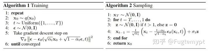
Then the optimization objective becomes

Predicting noise and predicting can be mathematically transformed into each other, but in practice, it is found that predicting noise performs better than predicting .

Note 1: However, from a mathematical intuition perspective, predicting noise is clearly better because is a rather complex distribution, while noise is merely a normal distribution.

Note 2: Some friends may wonder: After going around in a circle, did we just learn a normal distribution generator? Can’t I generate normal distribution without learning? Please note: In this article, all bold letters represent a specific sample value, not a random variable. We are not predicting any random noise value; we are predicting the specific value that transforms from a specific value to the corresponding value . Indeed this value is a sample drawn from the standard normal distribution , but we are not concerned with this distribution; we are only concerned with this specific sample value. In other words, this model is fundamentally a sampler that can draw corresponding values from the standard normal distribution based on input (Recall that GAN and VAE are also probability distribution samplers, just using different learning methods).

The overall training and inference process is shown in the figure below. Each training step randomly selects a to perform, as long as it ensures that the distribution of is uniform.

Modeling Under the SDE Framework

The above content, using DDPM as an example, provides a basic overview of the entire process of Diffusion. Now we hope to approach from a higher perspective, modeling the process of Diffusion from the perspective of SDE (Stochastic Differential Equations).

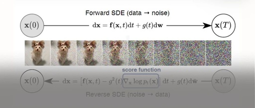
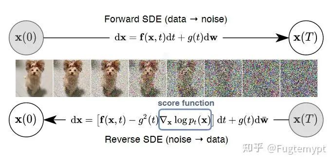
We regard the forward process as a differentiable stochastic process (Ito process, named after the Japanese mathematician Kiyoshi Ito, who completed this part of the theory), meaning it satisfies

Where represents the Wiener process (used to describe the stochastic process of Brownian motion).

Note: To fully understand this equation, one needs to supplement knowledge of stochastic processes and stochastic calculus. Here is a way to intuitively understand: a stochastic process about time is usually not differentiable. This is because the definition of differentiability is , but the stochastic variable at remains a random variable, which has a small probability of becoming very large, making the notation of small quantities inapplicable. Therefore, we need to introduce a differential quantity that adapts to the differentiation of random variables, and the Wiener process, as the simplest stochastic process, can meet our requirements well (this means we regard the normal distribution as the “1” in the world of random variables).

Thus we reconsider the calculation of each step in the forward process; in discrete form, each step is , while in continuous form, each step should be , which can be written in the format of (25)

Where .

Note: If you have not studied the Wiener process, you need to know (it is recommended to study it).

Then the probability distribution of the forward process can be written as

Using Bayes’ theorem, we can also obtain the probability distribution of the backward process

According to the Ito lemma (Taylor expansion of functions of random variables), we know

Thus the above expression can be rewritten as

Note that in the backward process, is known, not . However, since , we can replace it directly while removing small quantities.

Writing it in terms of probability distributions gives

Transforming it into Ito integral form gives

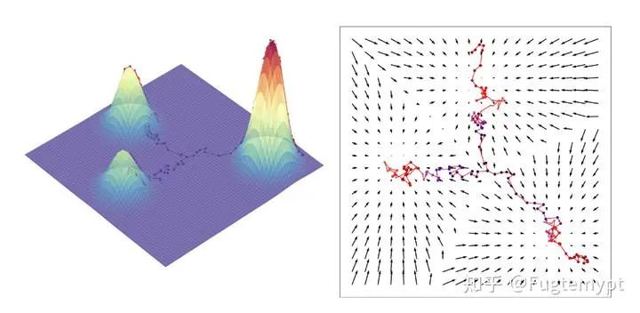
In the above expression, and are coefficients we define, and the only unknown quantity is , which is precisely what we fit using the neural network. Mathematically, it assigns a gradient to each point in the probability space; by following this gradient, we can reach the optimization target of .

Any different Diffusion model is actually just the result of using different and in (32).

Reply “Dataset” in the official account to get 100+ resources organized from various deep learning directions