Summary of Mathematical Principles Behind Graph Neural Networks

Original Link: https://rish-16.github.io/posts/gnn-math/

Graph Deep Learning (GDL) has been rapidly evolving for years. Many real-world problems make GDL a universal tool: it shows great promise in social media, drug discovery, chip implantation, prediction, bioinformatics, etc.

This article provides a detailed overview and explanation of popular Graph Neural Networks (GNNs) and their mathematical nuances. The underlying idea of graph deep learning is to learn the structural and spatial features of graphs with nodes and edges, where these nodes and edges represent entities and their interactions.

Graph

Before we dive into Graph Neural Networks, let’s first explore what a graph is in computer science.

A graph G(V,E) is a data structure that consists of a set of vertices (nodes) i ∈ V and a set of edges eij ∈ E that connect vertices i and j. If there is a connection between two nodes i and j, then eij = 1; otherwise, eij = 0. The connection information can be stored in an adjacency matrix A:

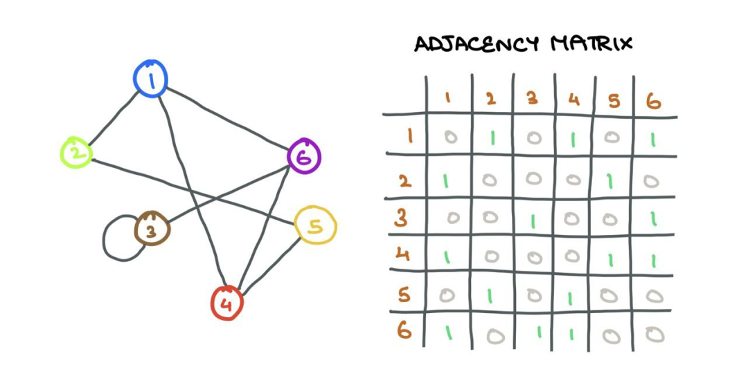
I assume the graphs in this article are unweighted (no edge weights or distances) and undirected (no directional association between nodes), and that these graphs are homogeneous (single type of nodes and edges; the opposite is “heterogeneous”).

The difference between graphs and regular data is that they have a structure that neural networks must respect; not utilizing it would be a waste. Below is an example of a social media graph, where nodes are users and edges are their interactions (like following/liking/sharing).

Connection with Images

For images, the image itself is a graph! This is a special variant called a “grid graph”, where for all internal nodes and corner nodes, the number of outward edges from a node is constant. There are some consistent structures in image grid graphs that allow simple convolution-like operations to be performed on them.

Images can be thought of as a special type of graph, where each pixel is a node and is connected to surrounding pixels by dashed lines. Of course, viewing images this way is impractical, as it implies a very large graph is needed. For example, a simple CIFAR-10 image of size 32×32×3 would have 3072 nodes and 1984 edges. For a larger ImageNet image of size 224×224×3, these numbers would be even larger.

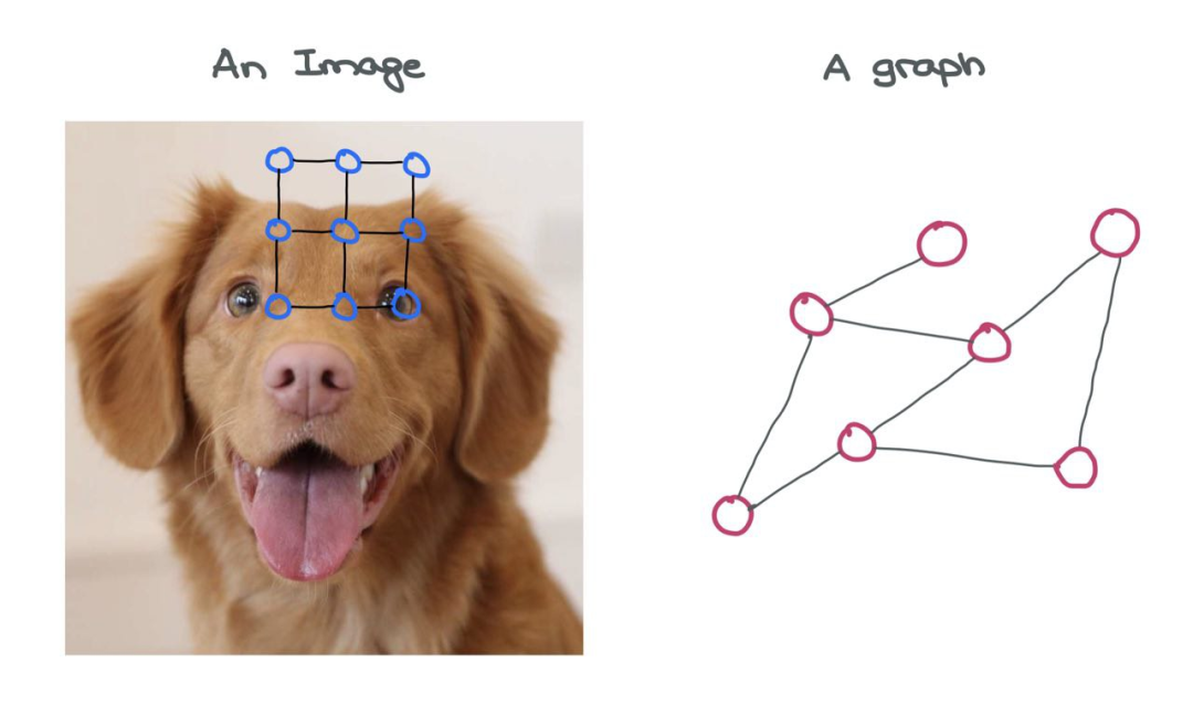
Compared to images, the different nodes in a graph have varying numbers of connections to other nodes and do not have a fixed structure, but it is this structure that adds value to the graph.

Graph Neural Networks

A single Graph Neural Network (GNN) layer consists of several steps performed at each node in the graph:

• Message Passing
• Aggregation
• Update

These form the building blocks for learning on graphs, and innovations in GDL occur through changes in these three steps.

Nodes

Nodes represent an entity or object, such as a user or an atom. Therefore, nodes have a set of attributes representing the entity. These node attributes form the features of the node (i.e., “node features” or “node embeddings”).

Typically, these features can be represented by vectors in R^d. This vector is either a latent dimensional embedding or constructed in a way where each entry is a different attribute of the entity.

For instance, in a social media graph, user nodes may have attributes such as age, gender, political inclination, relationship status, etc., which can be represented numerically. In a molecular graph, atom nodes may have chemical properties, such as affinity for water, force, energy, etc., which can also be represented numerically.

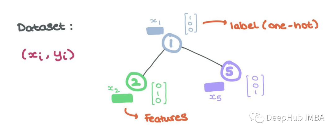
These node features are the input to the GNN, where each node i has associated node features x_i ∈ R^d and labels y_i (which can be continuous or discrete, similar to one-hot encoding).

Edges

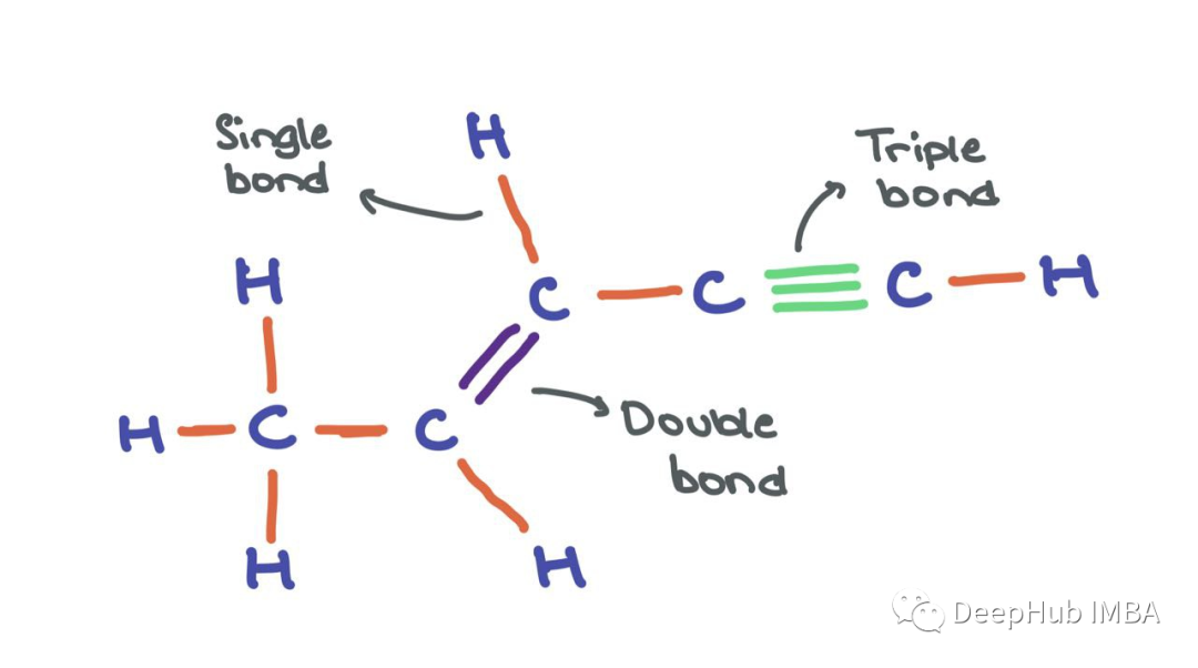
Edges can also have features a_ij ∈ R^d, for example, in cases where edges are meaningful (like chemical bonds between atoms). We can think of the following molecule as a graph where atoms are nodes and bonds are edges. While atom nodes themselves have their respective feature vectors, edges can have different edge features encoding different types of bonds (single, double, triple). However, for simplicity, I will omit edge features in this article.

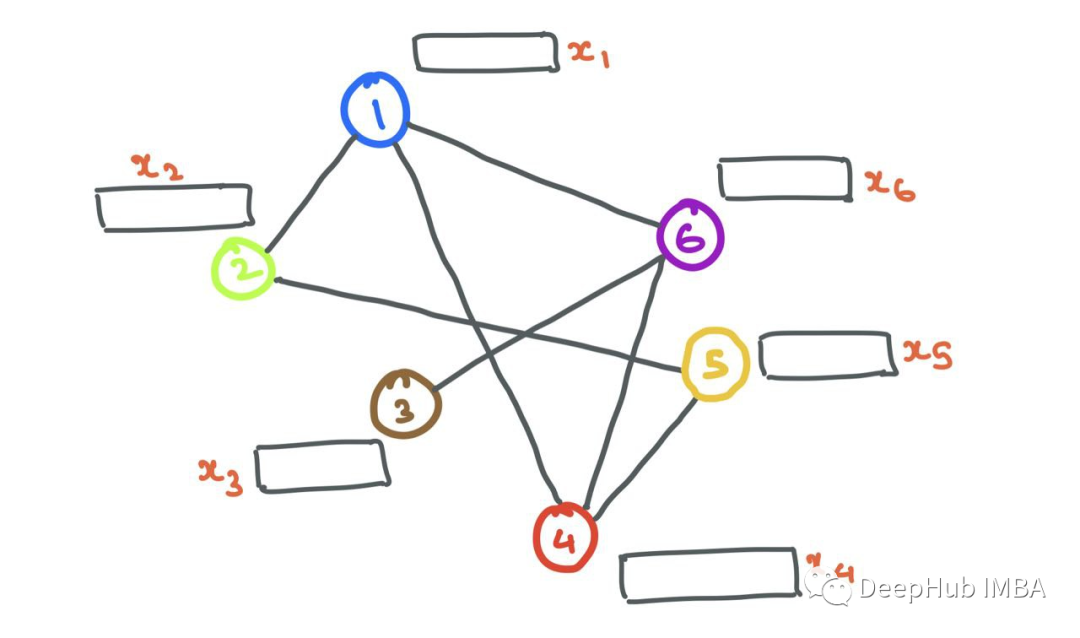
Now that we know how to represent nodes and edges in a graph, let’s start with a simple graph that has a bunch of nodes (with node features) and edges.

Message Passing

GNNs are known for their ability to learn structural information. Generally, nodes with similar features or attributes are connected (like in social media). GNNs learn how specific nodes are connected and why, by looking at the neighborhood of the node.

The neighbors N_i of node i are defined as the set of nodes j that are connected to i through edges. Formally, N_i = {j: e_ij ∈ E}.

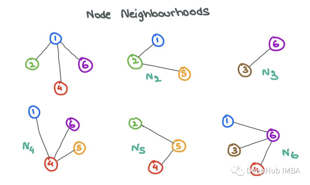
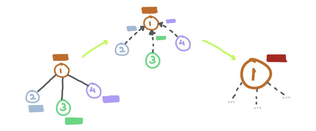
A person is influenced by their circle. Similarly, GNNs can learn a lot about node i by looking at the nodes in its neighborhood N_i. To facilitate this information sharing between the source node i and its neighbor nodes j, GNNs perform message passing.

For a GNN layer, message passing is defined as the process of obtaining the node features of neighbors, transforming them, and “passing” them to the source node. This process is repeated in parallel for all nodes in the graph. Thus, at the end of this step, all neighborhoods will have been checked.

Let’s zoom in on node 6 and examine its neighborhood N₆ = {1,3,4}. We take the node features x₁, x₃, and x₄, transform them with a function F, where F can be a simple neural network (MLP or RNN) or an affine transformation F(x_j) = W_j ⋅ x_j + b. Simply put, the “message” is the transformed node features coming from the source node.

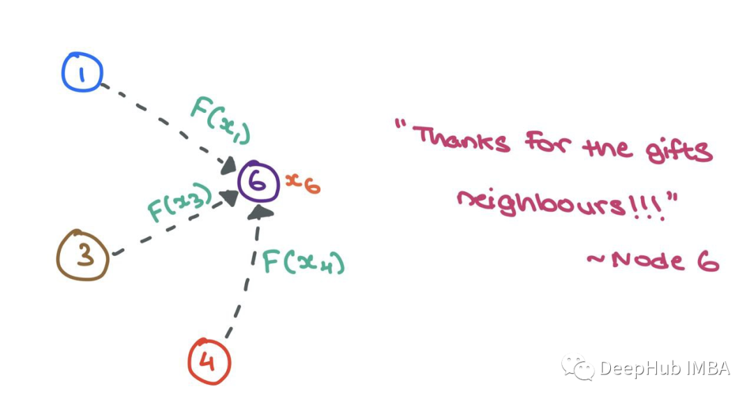
F can be a simple affine transformation or a neural network. Now let’s set F(x_j) = W_j ⋅ x_j for convenience of computation, where ⋅ represents simple matrix multiplication.

Aggregation

Now we have the transformed messages {F(x₁), F(x₃), F(x₄)} passed to node 6, and we must aggregate (“combine”) them somehow. There are many ways to combine them. Common aggregation functions include:

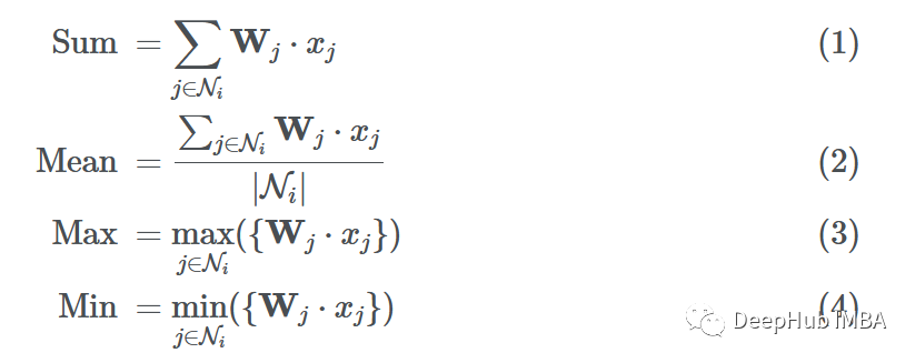
Assuming we use function G to aggregate the neighbors’ messages (using sum, mean, max, or min). The final aggregated message can be represented as:

Update

Using these aggregated messages, the GNN layer updates the features of the source node i. By the end of this update step, the node should not only know itself but also be aware of its neighbors. This is achieved by taking the feature vector of node i and combining it with the aggregated messages, which can be done with a simple addition or concatenation operation.

Using addition:

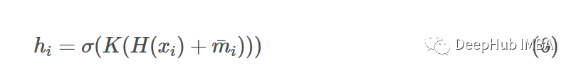
Where σ is an activation function (ReLU, ELU, Tanh), H is a simple neural network (MLP) or affine transformation, and K is another MLP that projects the addition vector into another dimension.

Using concatenation:

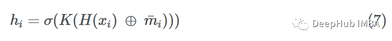
To further abstract this update step, we can view K as some projection function that transforms the messages and the source node embedding together:

The initial node features are denoted as x_i, and after passing through the first GNN layer, we transform the node features to h_i. Assuming we have more GNN layers, we can denote the node features as h_li, where l is the current GNN layer index. Similarly, it is evident that h_0i = x_i (i.e., the input to the GNN).

Putting It All Together

Now that we have completed the message passing, aggregation, and update steps, let’s combine them into a single GNN layer for a single node i:

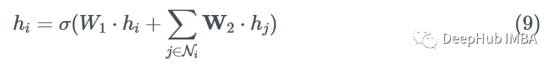
Here we use sum aggregation and a simple feedforward layer as functions F and H. Let h_i ∈ R^d, W₁, W₂ ⊆ R^d’ × d where d’ is the embedding dimension.

Using the Adjacency Matrix

So far, we have observed the entire GNN forward pass from the perspective of a single node i, but it’s also important to know how to implement GNN forward passes when given the entire adjacency matrix A and all node features X ⊆ R^N × d for N = ||V||.

In MLP forward passes, we want to weight the items in the feature vector x_i. This can be seen as the dot product of the node feature vector x_i ∈ R^d and the parameter matrix W ⊆ R^d’ × d, where d’ is the embedding dimension:

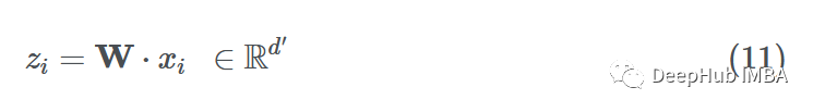
If we want to do this for all samples in the dataset (vectorized), we can simply multiply the parameter matrix with the feature matrix to get the transformed node features (messages):

In GNNs, for each node i, the message aggregation operation includes obtaining the feature vectors of neighboring nodes, transforming them, and summing them (in the case of sum aggregation).

For a single row A_i for each index j where A_ij = 1, we know that nodes i and j are connected → e_ij ∈ E. For example, if A₂ = [1,0,1,1,0], we know that node 2 is connected to nodes 1, 3, and 4. Thus, when we multiply A₂ with Z = XW, we only consider columns 1, 3, and 4 while ignoring columns 2 and 5:

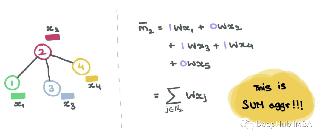
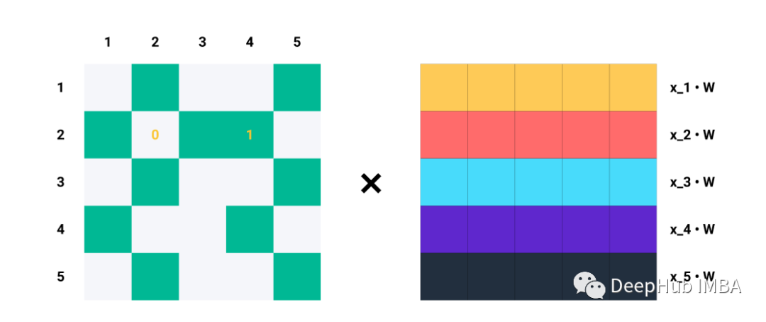
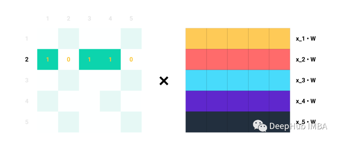
For instance, the second row of A.

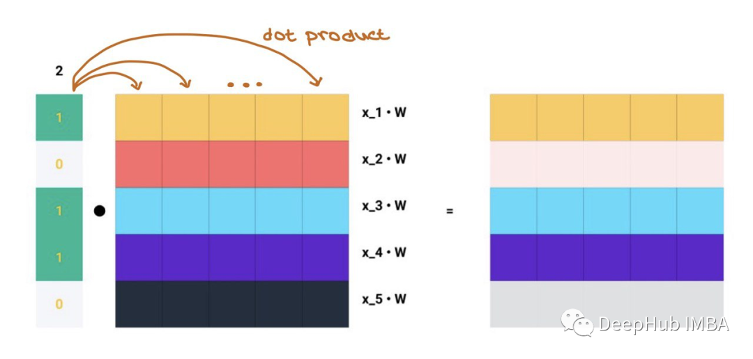
The matrix multiplication means the dot product of each row in A with each column in Z, which is the meaning of message aggregation!!

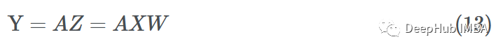
To obtain aggregated messages for all N, perform matrix multiplication of the entire adjacency matrix A with the transformed node features:

However, there is a small issue: the observed aggregated messages do not consider the feature vector of node i itself (as we did above). So we will add self-loops to A (each node i connects to itself).

This means the diagonal values need to be modified, and with some linear algebra, we can do this using the identity matrix!

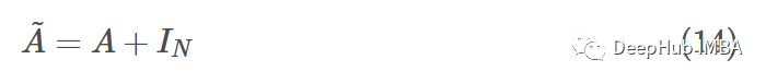
Adding self-loops allows GNNs to aggregate the features of the source node with its neighboring nodes’ features!!

With this, you can implement GNN propagation using matrices rather than single nodes.

⭐ To perform mean aggregation, we can simply divide the sum by the number of neighbors. For the above example, since A₂ = [1,0,0,1,1] has three 1s, we can divide ∑_j∈N2 Wx_j by 3, but it’s impossible to implement max (max) and min aggregation using the GNN adjacency matrix formula.

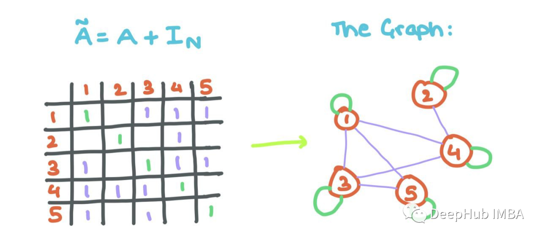
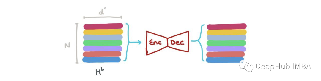
Stacking GNN Layers

Now that we have introduced how a single GNN layer works, how do we build an entire “network” using these layers? How does information flow between layers, and how does GNN refine the embeddings/representations of nodes (and/or edges)?

• The input to the first GNN layer is node features X ⊆ R^N × d. The output is intermediate node embeddings H₁ ⊆ R^N × d₁, where d₁ is the dimension of the first embedding. H₁ consists of h_1i: 1 → N ∈ R^d₁.
• H₁ is the input to the second layer. The next output is H₂ ⊆ R^N × d₂, where d₂ is the dimension of the second layer’s embedding. Similarly, H₂ consists of h_2i: 1 → N ∈ R^d₂.

• After several layers, at the output layer L, the output is H_L ⊆ R^N × d_L, where H_L consists of h_Li: 1 → N ∈ R^d_L.

The choice of {d₁, d₂, …, d_L} is entirely up to us and can be seen as hyperparameters of the GNN. Think of these as the number of units (“neurons”) chosen for the MLP layers.

Node features/embeddings (“representations”) are passed through the GNN. While the structure remains unchanged, the node representations continuously evolve across layers. Edge representations will also change but will not alter the connections or directions.

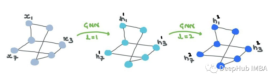
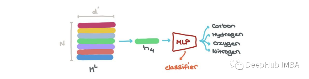
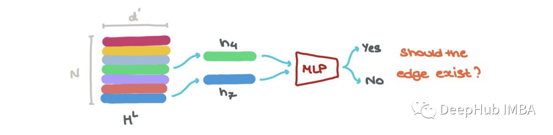
H_L can also do several things:

We can sum it along the first axis (i.e., ∑_Nk=1 h_Lk) to get a vector in R^d_L. This vector is the latest dimensional representation of the entire graph. It can be used for graph classification (e.g., what is this molecule?).

We can concatenate vectors in H_L (i.e., ⨁_Nk=1 h_k, where ⊕ is the vector concatenation operation) and pass it to a Graph Autoencoder. This operation is needed when the input graph has noise or damage, and we want to reconstruct a denoised graph.

We can perform node classification → what class does this node belong to? The nodes embedded at a specific index h_Li (i:1→N) can be classified into K classes (e.g., is this a carbon atom, hydrogen atom, or oxygen atom?).

We can also perform link prediction → is there a link between node i and j? The node embeddings h_Li and h_Lj can be input into another sigmoid-based MLP that outputs the probability that there is an edge between these nodes.

These are the operations GNNs perform in various applications. Regardless of the method, each h₁→N ∈ H_L can be stacked and seen as a batch of samples. We can easily treat it as a batch process.

For a given node i, the GNN aggregation at layer l has the l-hop neighborhood of node i. The node sees its immediate neighbors and delves into the network to interact with its neighbors’ neighbors.

This is why for very small, sparse (few edges) graphs, a large number of GNN layers often leads to performance degradation: because the node embeddings converge to a single vector as each node sees many nodes far away. This is ineffective for small graphs.

This also explains why most GNN papers often use ≤4 layers in experiments to prevent the network from encountering problems.

Training GNN with Node Classification as an Example.

During training, predictions can be made for nodes, edges, or the entire graph, using loss functions (e.g., cross-entropy) compared with ground-truth labels from the dataset. In other words, GNNs can be trained end-to-end using backpropagation and gradient descent.

Training and Test Data

Just like conventional ML, graph data can also be split into training and testing. There are two methods:

1. Transductive

Both training and testing data are in the same graph. Nodes in each set are connected. Only during training are the labels of test nodes hidden, while the labels of training nodes are visible. However, the features of all nodes are visible to the GNN.

We can perform binary masking for all nodes (if a training node i is connected to a test node j, simply set A_ij = 0 in the adjacency matrix).

Both training and testing nodes are part of the same graph. Training nodes expose their features and labels, while testing nodes only expose their features. Testing labels are hidden from the model. A binary mask is needed to tell the GNN which nodes are training nodes and which are testing nodes.

2. Inductive

The other approach involves separate training and testing graphs. This is similar to conventional ML, where the model only sees features and labels during training and only sees features for testing. Training and testing occur on two separate graphs. These testing graphs are distributed externally to check the generalization quality during training.

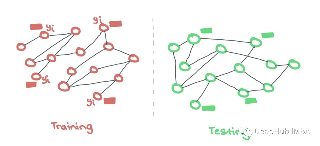
Just like conventional ML, training and testing data are stored separately. GNNs only use features and labels from training nodes. There is no need for a binary mask to hide test nodes as they come from different sets.

Backpropagation and Gradient Descent

During training, once we pass forward through the GNN, we obtain the final node representation h_Li ∈ H_L. To train in an end-to-end manner, we can do the following:

• Input each h_Li into an MLP classifier to get predictions ^y_i;
• Calculate the loss using ground-truth y_i and predicted y_i → J(y_i, y_i);
• Use backpropagation to compute ∂J/∂W_l, where W_l is the parameter matrix from layer l;
• Use the optimizer to update the parameters W_l in each layer of the GNN;

• (If needed) we can also fine-tune the weights of the classifier (MLP) network.

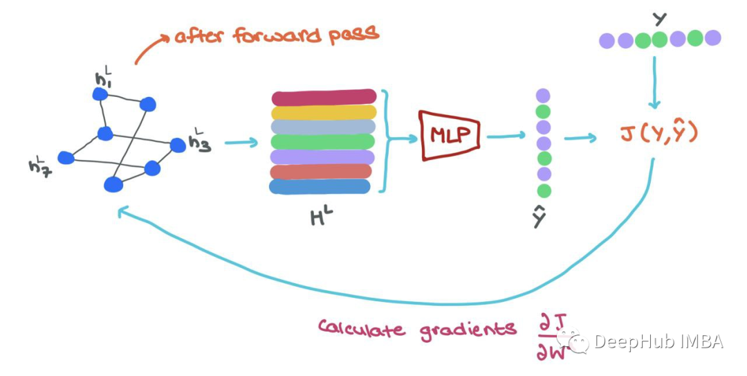
🥳 This means that GNNs are easy to parallelize in both message passing and training. The entire process can be vectorized (as shown above) and executed on GPUs!!

Popular Graph Neural Networks Summary

We have introduced the basic processes of ancient neural networks; now let’s summarize popular graph neural networks and break down their equations and mathematics into the three GNN steps mentioned above. Many architectures combine the message passing and aggregation steps into one function rather than executing them explicitly one after the other, but for mathematical convenience, we will try to break them down and view them as a single operation!

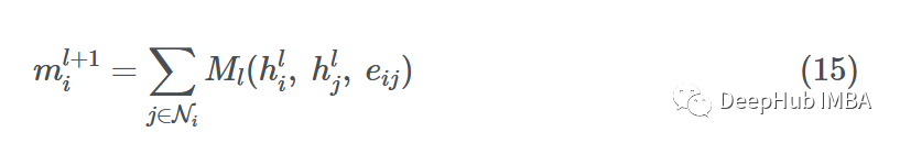
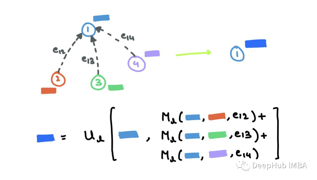
1. Message Passing Neural Networks

https://arxiv.org/abs/1704.01212

Message Passing Neural Networks (MPNN) decompose the forward pass into a message passing phase with a message function M_l and a readout phase with a vertex update function U_l.

MPNN combines the message passing and aggregation steps into a single message passing phase:

The readout phase is the update step:

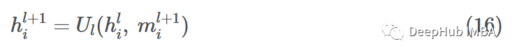
Where m_l+1v is the aggregated message, and h_l+1v is the updated node embedding. This is very similar to the process I mentioned above. The message function M_l is a mix of F and G, and function U_l is k, where e_ij denotes possible edge features, which may also be omitted.

2. Graph Convolution

https://arxiv.org/abs/1609.02907

Graph Convolutional Networks (GCNs) study the entire graph in the form of an adjacency matrix. Adding self-connections to the adjacency matrix ensures that all nodes are connected to themselves to obtain ~A. This ensures that the source node’s embedding is considered during message aggregation. The combined message aggregation and update steps are as follows:

Where W_l is a learnable parameter matrix. Here, X is replaced by H to generalize the node features at any layer l, where H₀ = X.

Due to the associative property of matrix multiplication (A(BC)=(AB)C), it does not matter in which order we multiply matrices (whether ~A is multiplied first, then W_l, or H_l is multiplied first, then ~A). Authors Kipf and Welling further introduced the degree matrix ~D as a form of