Machine Heart Column
This column is produced by Machine Heart SOTA! Model Resource Station, updated every Sunday on the Machine Heart public account.
This column will review common tasks in natural language processing, computer vision, and other fields, and detail the classic models that have achieved SOTA on these tasks. Visit SOTA! Model Resource Station (sota.jiqizhixin.com) to access the implementation code, pre-trained models, and APIs included in this article.
This article will be serialized in 2 issues, covering 19 classic models that have achieved SOTA in speech synthesis.
-
Issue 1: BLSTM-RNN, WaveNet, SampleRNN, Char2Wav, Deep Voice, Parallel WaveNet, GAN, Tacotron, VoiceLoop
-
Issue 2: Tacotron2, GST, DeepVoice3, ClariNet, LPCNet, Transformer-TTS, Glow-TTS, Flow-TTS, cVAE+Flow+GAN, PnG BERT
You are reading Issue 1. Visit SOTA! Model Resource Station (sota.jiqizhixin.com) to access the implementation code, pre-trained models, and APIs included in this article.
Overview of Models Included in This Issue
| Model | SOTA! Model Resource Station Inclusion Status | Source Paper |
|---|---|---|
| BLSTM-RNN | https://sota.jiqizhixin.com/project/blstm-rnn | TTS Synthesis with Bidirectional LSTM based Recurrent Neural Networks |
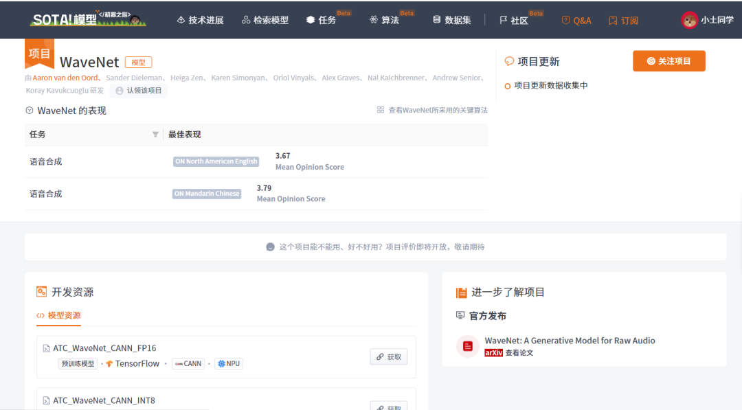
| WaveNet | https://sota.jiqizhixin.com/project/wavenet-2, Number of Implementations: 7, Supported Frameworks: PyTorch, TensorFlow, etc. | WaveNet: A Generative Model for Raw Audio |
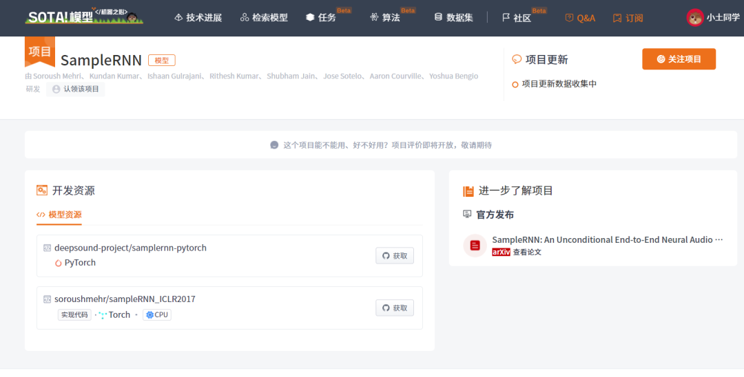
| SampleRNN | https://sota.jiqizhixin.com/project/samplernn, Number of Implementations: 2, Supported Frameworks: PyTorch, Torch | SampleRNN: An Unconditional End-to-End Neural Audio Generation Model |
| Char2Wav | https://sota.jiqizhixin.com/project/char2wav | Char2Wav: End-to-end speech synthesis |
| Deep Voice | https://sota.jiqizhixin.com/project/deep-voice, Number of Implementations: 1, Supported Framework: PyTorch | Deep Voice: Real-time Neural Text-to-Speech |
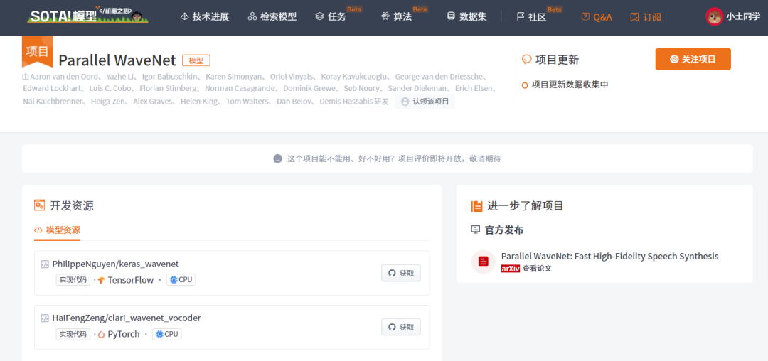
| Parallel WaveNet | https://sota.jiqizhixin.com/project/parallel-wavenet, Number of Implementations: 2, Supported Frameworks: PyTorch, TensorFlow | Parallel WaveNet: Fast High-Fidelity Speech Synthesis |
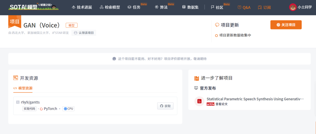
| GAN | https://sota.jiqizhixin.com/project/gan-voice, Number of Implementations: 1, Supported Framework: PyTorch | Statistical Parametric Speech Synthesis Using Generative Adversarial Networks Under A Multi-task Learning Framework |
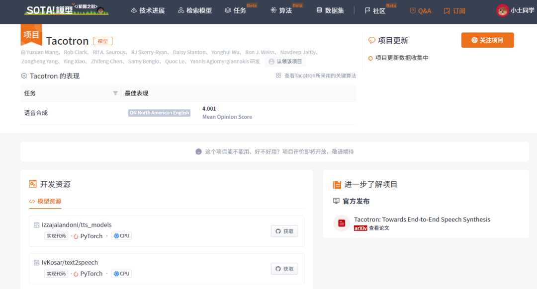
| Tacotron | https://sota.jiqizhixin.com/project/tacotron, Number of Implementations: 23, Supported Frameworks: PyTorch, TensorFlow | Tacotron: Towards End-to-End Speech Synthesis |
| VoiceLoop | https://sota.jiqizhixin.com/project/voiceloop | VoiceLoop: Voice Fitting and Synthesis via a Phonological Loop |
Speech synthesis refers to the technology that generates synthetic speech through mechanical or electronic methods. Text To Speech (TTS) converts text into human-like speech (input is text for speech synthesis), which is a typical and well-known speech synthesis task. Speech synthesis is widely applicable in business scenarios such as intelligent customer service, audio reading, news broadcasting, and human-computer interaction. Speech synthesis and speech recognition technologies are two key technologies necessary for achieving human-computer voice communication and establishing a spoken system with listening and speaking capabilities. Enabling computers to have speech abilities similar to humans is an important competitive market in today’s information industry. Compared to speech recognition, speech synthesis technology is relatively more mature and has begun to successfully move towards industrialization, with large-scale applications on the horizon. Companies like iFlytek and Volcano Engine are examples of the industrialization of speech synthesis technology.Traditional speech synthesis models (also known as Statistical Parametric Speech Synthesis (SPSS)) include three processing steps: front-end processing – acoustic model – vocoder, where both the front-end processing and vocoder have some common schemes, and the main improvement points for different tasks are primarily in the acoustic model part. The front-end processing mainly refers to the analysis of text, usually preprocessing the text input into the speech synthesis system, such as converting it into a phoneme sequence, and sometimes performing sentence segmentation, prosody analysis, etc., ultimately extracting voice and prosody from the text. The acoustic model mainly generates acoustic features based on linguistic features. Finally, the vocoder synthesizes speech signals based on the acoustic features. Building these modules requires a lot of expertise and complex engineering implementation, which will require substantial time and effort. Additionally, incorrect combinations of each component may make the model difficult to train. Introducing deep learning models (DNN) into the traditional three-stage speech synthesis model can learn the mapping function from linguistic features (input) to acoustic features (output). DNN-based acoustic models provide effective distributed representations for the complex dependencies between linguistic features and acoustic features. However, one limitation of the acoustic feature modeling method based on feedforward DNN is that it ignores the continuity of speech. DNN-based methods assume that each frame is independently sampled, even though there are correlations between consecutive frames in speech data. Recurrent Neural Networks (RNNs) provide an effective way to model the correlations between adjacent frames of speech, as they can use all available input features to predict the output features of each frame. On this basis, some researchers have replaced DNNs with RNNs to capture the long-term dependencies of speech frames to improve the quality of synthesized speech.In recent years, with the rise of deep learning, model accuracy has made significant advancements. Among them, the powerful feature learning capabilities of deep neural networks greatly simplify the feature extraction process and reduce the modeling’s reliance on expert experience. The modeling process has gradually shifted from the previously complex multi-step process to a simple end-to-end modeling process, making end-to-end neural network speech synthesis the mainstream method for industrial-scale applications. End-to-end models can be seen as having two main stages: acoustic model modeling and neural vocoder. Among them, the acoustic model modeling directly converts the input text/phoneme sequence into frame-level speech features, while the neural vocoder converts frame-level speech features into speech waveforms, which includes both autoregressive and non-autoregressive models. End-to-end methods outperform traditional methods in terms of performance and deployment scalability.
BLSTM-RNN
This model uses a recurrent neural network (RNN) with Bidirectional Long Short-Term Memory (BLSTM) units to capture the correlations or co-occurrences of any two moments in the speech corpus, used for parameterizing TTS tasks (Statistical Parametric TTS Synthesis system), and belongs to the application of deep learning models in the front-end processing of speech synthesis. At the temporal scale, RNNs can be unfolded into a broad structure by taking the previous or next latent state. Like DNNs, RNNs can also be stacked in multiple layers and have a deep structure in space.
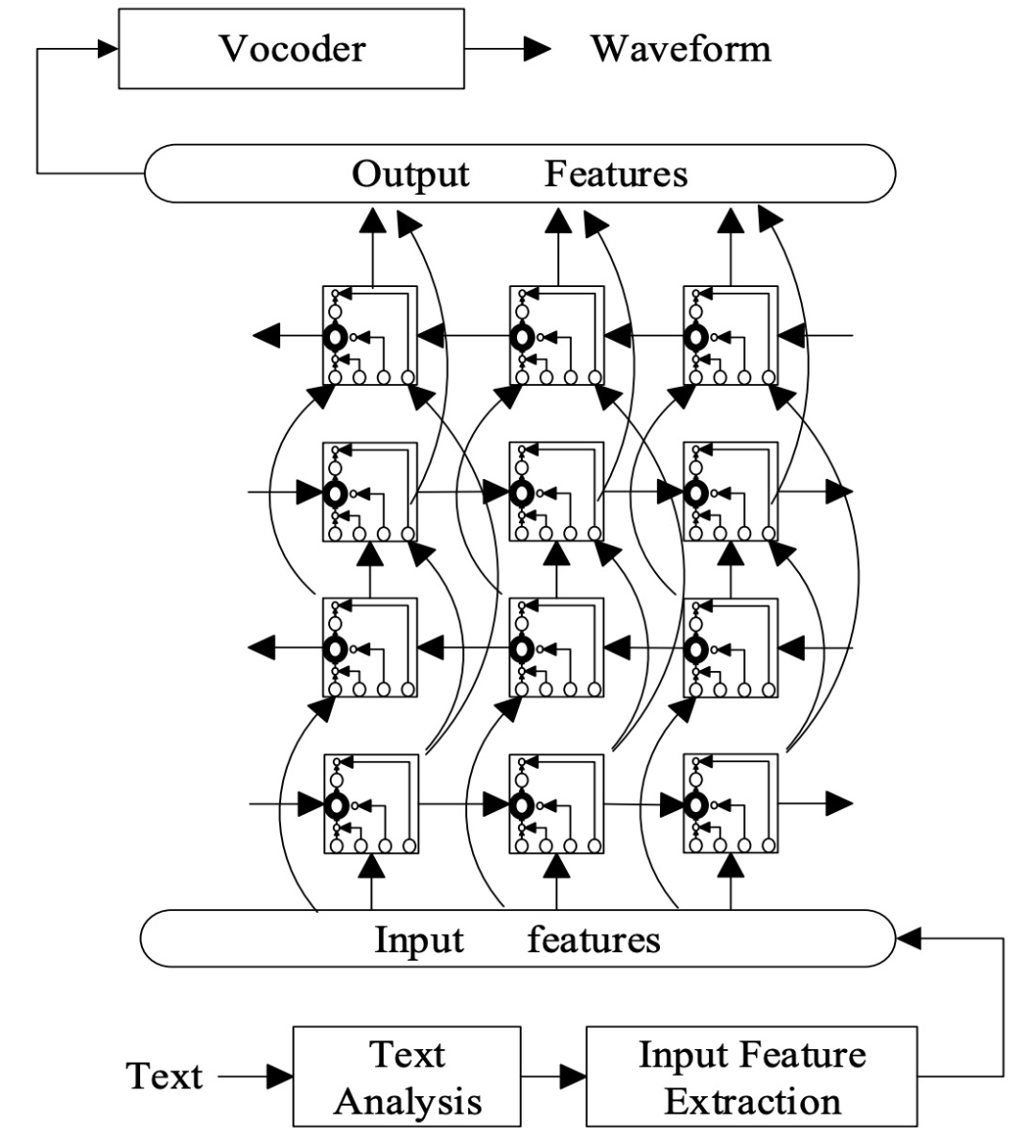
Figure 1. TTS synthesis based on BLSTM-RNN
In TTS synthesis based on BLSTM-RNN, rich context is also used as input features, which include binary features for categorical context, such as phone labels, POS tags of the current word, and TOBI labels, as well as numerical features for numerical context, such as the number of words in a phrase or the position of the current phone’s current frame. The output features are acoustic features such as spectral envelope and fundamental frequency. Input and output features can be temporally aligned frame by frame through a trained HMM model. RNNs are also powerful, making it possible to model sequential data with unordered input-output arrangements. The weights of DNNs are trained by minimizing the error between the mapping output and target output given the input, using pairs of input and output features extracted from the training data. In RNN training, the training criterion is to minimize the mean square error between the output features and the ground truth. Back-propagation through time (BPTT) is the most commonly used algorithm for training RNNs. BPTT unfolds the RNN into a feedforward network over time, and then trains the unfolded network using backpropagation. For deep bidirectional LSTMs, the BPTT algorithm is applied simultaneously to the forward and backward latent nodes and backpropagates layer by layer. In DNN training, weights are trained using backpropagation and a mini-batch-based stochastic gradient descent algorithm, which randomly selects mini-batches of frames from the entire training set. In RNN training, the weight gradients are computed over the entire corpus. To parallelize and accelerate, dozens of corpora are randomly selected for each update, which are then used to simultaneously update the weights of the RNN. During the synthesis process, the input text is first converted into input feature vectors through text analysis, and then the input feature vectors are mapped to output vectors through the trained BLSTM-RNN. In HMM-based TTS, the corresponding context labels are used to access decision trees to obtain the HMM state sequence of the context. The means and covariances of the corresponding HMM states are sent to the parameter generation module to generate smooth speech parameter trajectories with dynamic information. In DNN-based TTS, the speech feature generation module can generate smooth trajectories of speech parameter features that satisfy the statistics of static and dynamic features by setting the DNN’s predicted output features as the mean vector of output features across all training data and pre-computed (global) variance, while voiced/unvoiced flags are determined by the empirical threshold predicted by the DNN. Considering RNN’s ability to model sequential problems, the parameter generation module is implicitly included in TTS synthesis based on DBLSTM-RNN, meaning that the output features of the RNN are simply static features: spectral envelope, gain, fundamental frequency, and U/V decisions, which are then directly input to the vocoder to synthesize the final speech waveform.
| Item | SOTA! Platform Project Details Page |
|---|---|
| BLSTM-RNN | Visit SOTA! Model Platform for implementation resources:https://sota.jiqizhixin.com/project/blstm-rnn |
WaveNet
WaveNet is a deep generative model of raw audio waveforms and belongs to the application of deep learning models in the front-end processing of speech synthesis, operating at the waveform level. WaveNet is a fully probabilistic autoregressive model, where the predicted distribution of each audio sample depends on all previous samples. WaveNet can be trained efficiently on audio data at sampling rates of tens of thousands per second. WaveNet also requires tuning existing TTS front-end linguistic features, so it is not an end-to-end method but rather replaces the vocoder and acoustic model. WaveNet employs causal convolution and dilated convolution:
Causal convolution ensures that the model’s output does not violate the order of the data, meaning that the prediction output at any moment does not depend on data from any future moment. During the training phase, the samples to be computed for the output at each moment are known, allowing for the conditional probability predictions at all moments to be computed in parallel. Since there are no recurrent connections in models that use causal convolution, they generally train faster than RNNs, especially for long sentences. One issue with causal convolution is that it requires many layers or a large convolution kernel to increase its receptive field. For example, in Figure 2, the receptive field is only 5 units (receptive field = number of layers + length of convolution kernel – 1). Therefore, WaveNet uses dilated convolution to increase the receptive field by several orders of magnitude without significantly increasing computational cost.
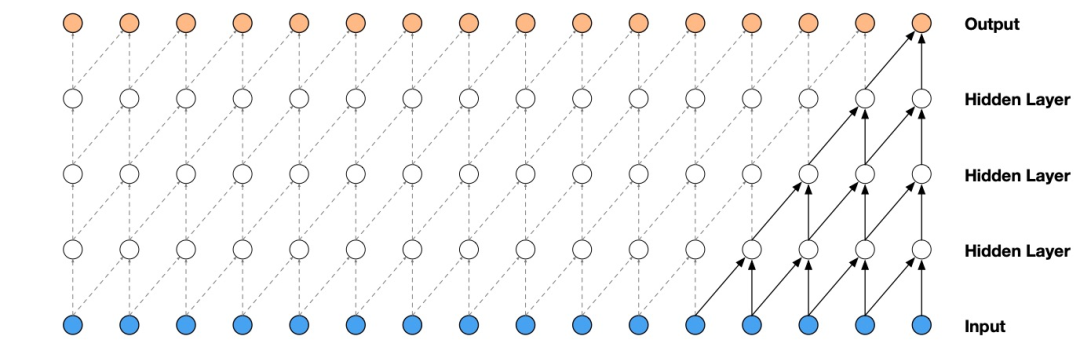
Figure 2. Visualization of causal convolution layer stacks
Dilated convolution is a convolution method that skips steps when convolving on data larger than itself. Compared to normal convolution, dilated convolution allows the network to perform coarse-grained convolution operations. As shown in Figure 3, the dilation factor of dilated convolution doubles each layer (1, 2, 4, 8), achieving a very large receptive field (16 units) with just a few layers. The maximum dilation factor in WaveNet reaches 512, yielding a receptive field of 1024 units.
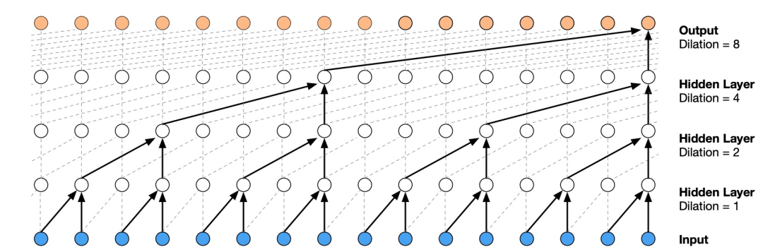
Figure 3. Visualization of dilated causal convolution layer stacks
Softmax Distribution:
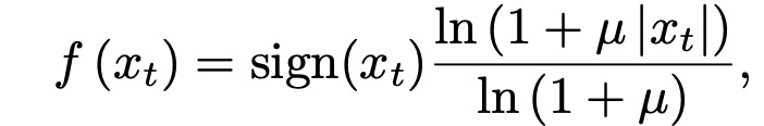
Raw audio is typically stored in 16Bit format, requiring the softmax layer to output 65536 possible values for each time step. For convenience and speed in computation, a µ-law compression transformation is applied to the data first, resulting in 256 quantized values. The µ-law compression transformation algorithm is as follows:
Gated Activation Units:
The gated activation units used in WaveNet are as follows:

Where ∗ represents the convolution operation, ⊙ represents the pointwise multiplication operation, σ(.) is the sigmoid function, k is the layer index, f and g are their respective filters and gates, and W is the learnable convolution kernel.Residual and Skip Connections:
WaveNet uses residual and skip connections to accelerate convergence and allow deeper model training. The structural schematic is as follows:
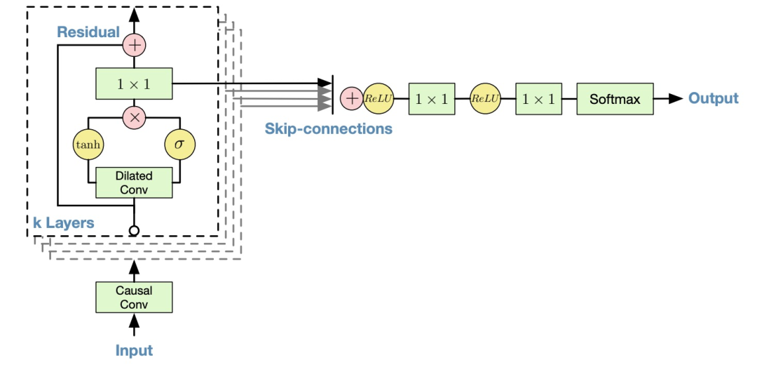
Figure 4. Overview of residual blocks and the entire architecture
Conditional WaveNet:
Given an additional input h, WaveNet can be conditioned on this input

Conditional modeling based on input variables allows WaveNet to generate audio with desired features. For instance, speaker identity can be used as a conditional input to WaveNet, which will then select that speaker’s voice for audio output.Context Stacks:
Several methods have been proposed to increase the receptive field size of WaveNet: increasing the dilation factor, using more layers, larger filters, larger dilation factors, or combinations thereof. An additional method is to use separate smaller context stacks to handle long-range information of the speech signal, forming a larger WaveNet that only processes a small portion of the audio signal (trimming at the end).
Multiple context stacks with different lengths and numbers of latent units can be used. The larger the receptive field of the stack, the fewer units per layer. Context stacks can also have pooling layers that operate at lower frequencies. This keeps computational demands at a reasonable level while being intuitively consistent with the capacity needed to model temporal correlations over longer time scales.
Currently, the SOTA! platform includes 7 model implementation resources for WaveNet.
| Item | SOTA! Platform Project Details Page |
|---|---|
WaveNet |
Visit SOTA! Model Platform for implementation resources:https://sota.jiqizhixin.com/project/wavenet-2 |
SampleRNN
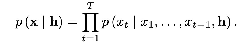
SampleRNN combines a memoryless module, i.e., autoregressive multilayer perceptrons, and stateful recurrent neural networks in a hierarchical manner, capable of capturing the latent sources of temporal variation across three datasets of different natures, belonging to the application of deep learning models in the front-end processing of speech synthesis. Since SampleRNN has different modules operating at different clock rates (contrary to WaveNet), it can flexibly allocate computational resources for modeling at different levels of abstraction. SampleRNN is a density model of audio waveforms. SampleRNN’s probability of the waveform sample sequence X={x1, x2, . . , xT} (the random variable of the input data sequence) is expressed as the product of the probabilities of each sample conditioned on all previous samples:
RNNs are typically used to model sequential data, which can be expressed as:
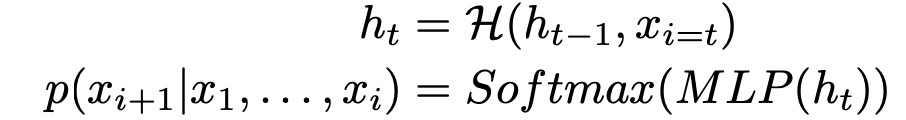
Where H is one of the known memory units, which can be a Gated Recurrent Unit (GRU), Long Short-Term Memory (LSTM), or its deep variations. However, modeling raw audio signals is challenging due to their very different scale structures: correlations exist between adjacent samples as well as between samples spaced thousands apart. SampleRNN helps address this challenge by using a hierarchical structure of modules, where each module operates at different temporal resolutions. The lowest module processes individual samples, while each higher module operates at increasing time scales and lower temporal resolutions. Each module adjusts to the one below it, with the lowest module outputting sample-level predictions. The entire hierarchical structure is jointly trained end-to-end via backpropagation.
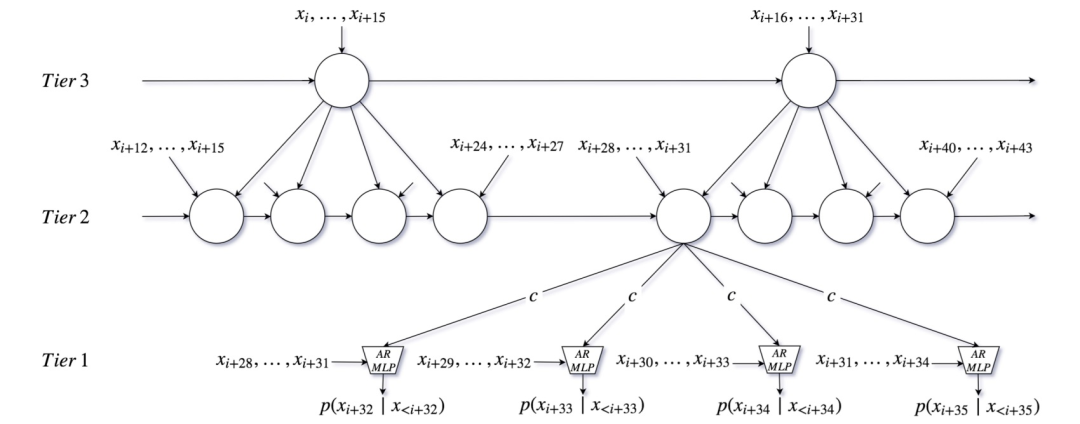
Figure 5. Snapshot of the unrolled model at time step i with K=3 layers. For simplicity, all layers use a single RNN and an upsampling rate of r=4
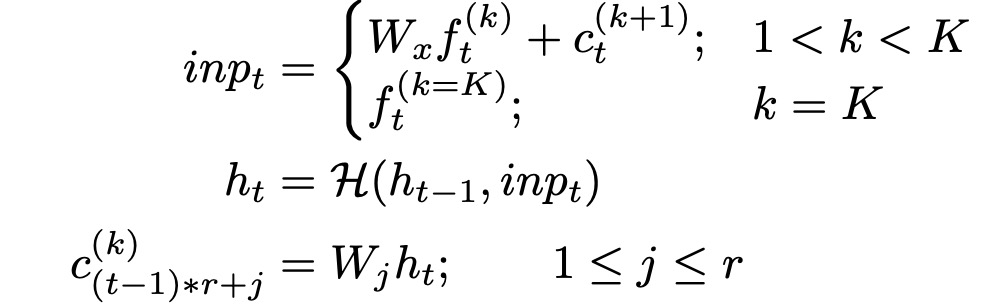
The higher-level modules in SampleRNN do not operate on individual samples but rather on non-overlapping frames of size F_S(k) (“frame size”) at level k in the hierarchy (frames are denoted as f(k)). Each frame-level module is a deep RNN that summarizes the history of its input into an adjustment vector for the next module to pass down. The condition for a variable number of frames up to time point t-1 is represented by a fixed-length latent state or memory (h_t)^(k), where t relates to the clock rate of that layer.RNN updates its memory at time point t as a function of the previous memory (h_t-1)^(k) and an input (inp_t)^(k). For the top layer k = K, this input is simply the input frame. For intermediate layers (1 < k < K), this input is a linear combination of the adjustment vector from the previous layer and the current input frame.Since different modules operate at different temporal resolutions, each module’s output vector c must be upsampled to a series of r^(k) vectors (where r^(k) is the ratio between the module’s temporal resolution) before being passed down to the next module’s input.This is accomplished with a set of r^(k) independent linear projections.
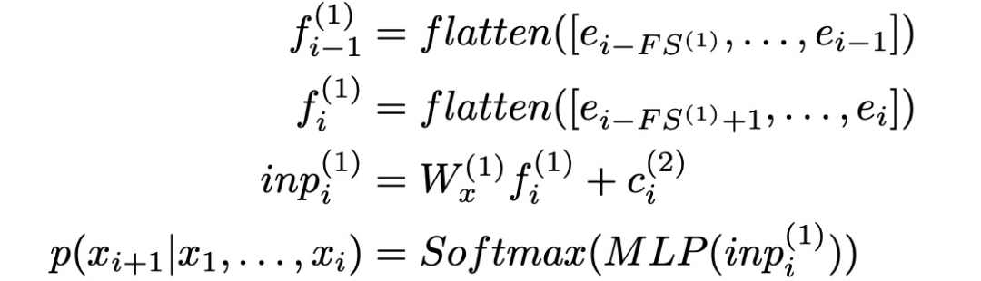
The lowest module (k=1 layer) in the SampleRNN hierarchy outputs a distribution over the sample x_i+1, conditioned on the previous FS^(1) samples and the vector (c_i)^(k=2) from the next higher module, which encodes the sequence information from the previous frames. Since F_S(1) is typically a small value, and the correlations between nearby samples can be easily modeled with a simple memoryless module, a multilayer perceptron (MLP) is used instead of an RNN, which slightly speeds up training. Assuming e_i represents x_i after embedding, the conditional distribution can be implemented as follows, and to clarify further, below are two consecutive sample-level frames:
Finally, using truncated backpropagation, each sequence is split into short subsequences, and gradients are only propagated to the beginning of each subsequence, allowing the recurrent model to be effectively trained.
Currently, the SOTA! platform includes 2 model implementation resources for SampleRNN.
| Item | SOTA! Platform Project Details Page |
|---|---|
| SampleRNN | Visit SOTA! Model Platform for implementation resources:https://sota.jiqizhixin.com/project/samplernn |
Char2Wav
Char2Wav consists of two parts: a reader and a vocoder. The reader comprises an encoder and a decoder, where the encoder is a bidirectional RNN that accepts text/phonemes as input, and the decoder is an attention-based RNN that generates the corresponding acoustic features for the vocoder. The standout contribution of Char2Wav is its ability to learn to produce wav directly from text. Char2Wav is an end-to-end model that can be trained to generate characters, using the SampleRNN neural vocoder to predict vocoder parameters. The structure of Char2Wav is shown in Figure 6.
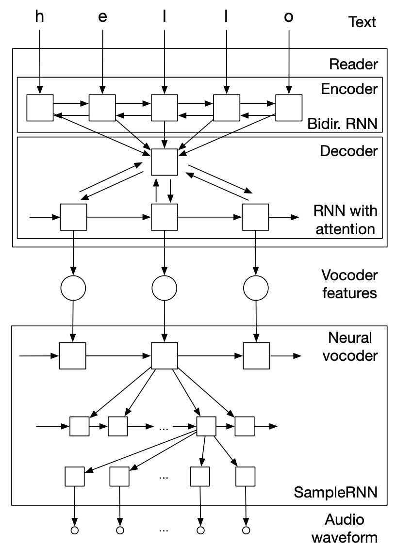
Figure 6. Char2Wav end-to-end speech synthesis model
Reader:
The attention-based recurrent sequence generator (ARSG) is a recurrent neural network that generates a sequence Y=(y1,…,yT) conditioned on the input sequence X, which is preprocessed by an encoder to output the sequence h=(h1,…,hL). In this work, the output Y is an acoustic feature sequence, and X is the text or phoneme sequence to be generated. Additionally, the encoder is a bidirectional recurrent network. In the i-th step, the ARSG focuses on h while generating yi:
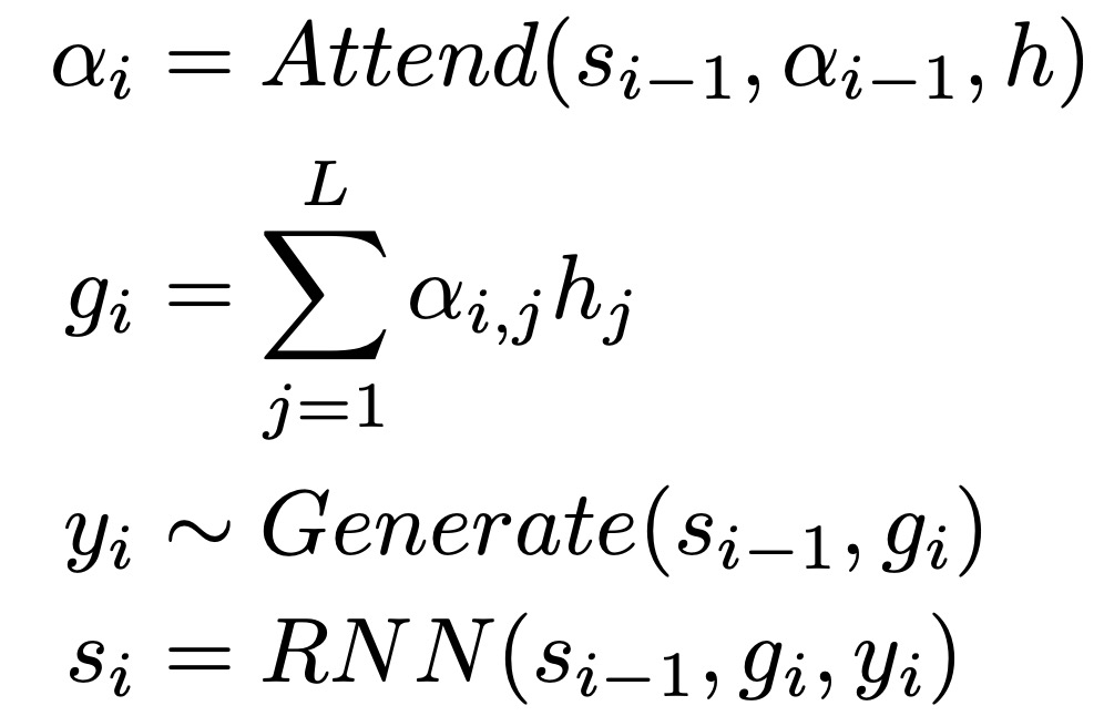
Where s_i-1 is the state of the generator recurrent neural network at the (i – 1)-th step, α_i∈R^L is the attention weight or arrangement. Using a location-based attention mechanism, α_i = Attend(s_i-1, α_i-1), given a conditional sequence h of length L, we have:
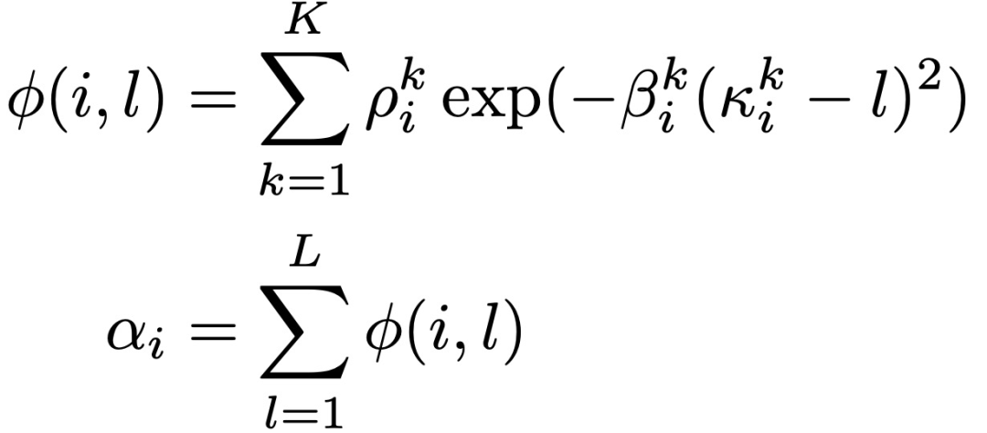
Where κi, βi, and ρi represent the position, width, and importance of the window, respectively. NEURAL VOCODER:
The quality of speech synthesis is limited by the vocoder, and to ensure high-quality output, SampleRNN is introduced. SampleRNN is used to model extremely long-term dependencies, where the vertical structure captures the dynamics of sequences at different times. Capturing long audio steps (word-level) and short audio steps’ long correlations is important. The conditional version model learns the mapping between vocoder feature sequences and corresponding audio samples, where the output at each time step depends on its vocoder features and the outputs of previous time steps.
| Item | SOTA! Platform Project Details Page |
|---|---|
| Char2Wav | Visit SOTA! Model Platform for implementation resources:https://sota.jiqizhixin.com/project/char2wav |
The Deep Voice system is a high-quality text-to-speech system completely built with deep neural networks. The system consists of 5 important components: a segmentation model for locating phoneme boundaries, a grapheme-to-phoneme conversion model, a phoneme duration prediction model, a fundamental frequency prediction model, and an audio synthesis model. Focusing on the segmentation task, a new method using deep neural networks for phoneme boundary detection is proposed, using the CTC (connectionist temporal classification) loss function. Focusing on the audio synthesis task, a variant of WaveNet is introduced that requires fewer parameters and trains faster than the original WaveNet. Neural networks are used in each component, making it simpler and more flexible than traditional TTS systems (which require manual tuning and a lot of expertise).
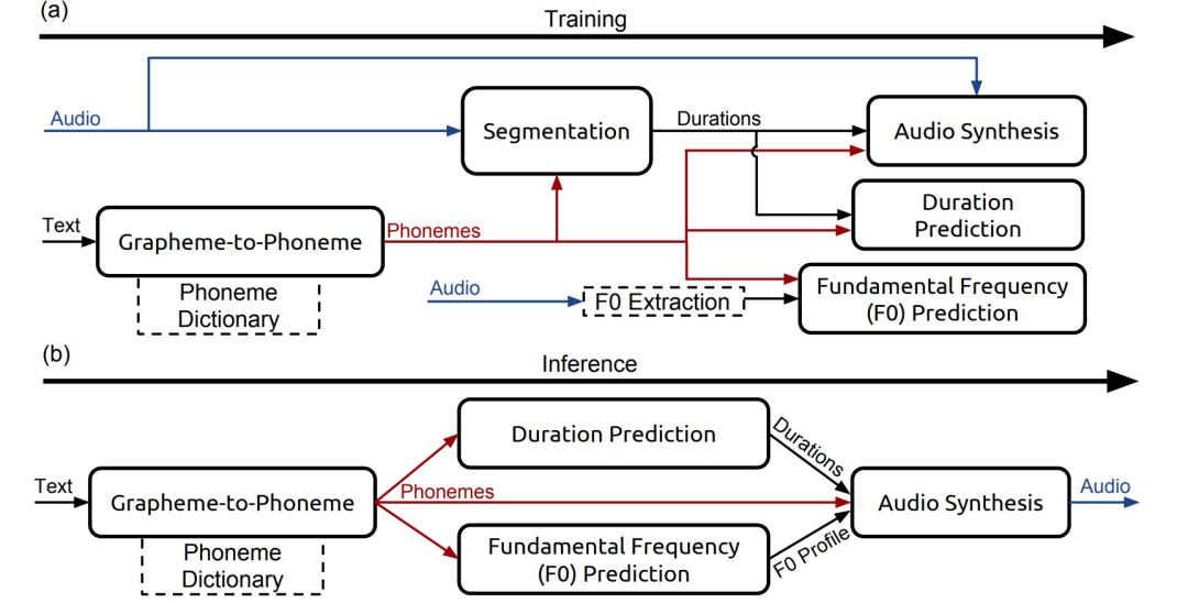
Figure 7. Structure of Deep Voice, (a) training program, (b) inference program, the left side is input, the right side is output. The duration prediction model and F0 prediction model are implemented by a single neural network trained with joint loss. The grapheme-to-phoneme model is used as a backup for words not present in the phoneme dictionary. The dashed line indicates non-learning components
Deep Voice is a speech synthesis system developed using DNNs, primarily replacing various modules in traditional parametric speech synthesis with neural networks, specifically including the following five modules: (1) grapheme-to-phoneme conversion model: converts the input text into a phoneme sequence; (2) segmentation model: locates phoneme boundaries; (3) phoneme duration model: predicts the duration of phonemes; (4) fundamental frequency model: predicts F0, whether the phoneme is voiced; where the phoneme duration model and fundamental frequency model are trained together; (5) audio synthesis model: synthesizes audio based on outputs from (1)/(3)/(4).
Grapheme-to-Phoneme Model:
The grapheme-to-phoneme model is based on an encoder-decoder structure. It uses a multi-layer bidirectional encoder with gated recurrent units (GRUs) as non-linearities and a unidirectional GRU decoder. The initial state of each decoding layer is initialized to the final latent state of the corresponding encoder’s forward layer. This architecture is trained with teacher forcing, and decoding is performed using beam search. Three bidirectional layers with 1024 units are used in the encoder, and three unidirectional layers of the same size in the decoder, with a beam width of 5. During training, a probability of 0.95 dropout is applied after each recurrent layer.
Segmentation Model:
A segmentation model is trained to achieve alignment between the given corpus and the target phoneme sequence. This task is similar to the alignment problem between speech and written output in speech recognition. In this domain, the CTC loss function has proven very suitable for character alignment tasks to learn the mapping between sound and text. Networks trained with CTC generate phoneme sequences and can generate short peaks for each output phoneme. The direct training results can make phonemes roughly consistent with audio, but they cannot detect precise phoneme boundaries. To overcome this problem, the network is trained to predict sequences of phoneme pairs rather than individual phonemes. The network then outputs phoneme pairs during the time period close to the boundaries of the two phonemes.
Phoneme Duration and Fundamental Frequency Model:
A single architecture is used to jointly predict phoneme duration and the fundamental frequency that varies over time. The input to this model is a phoneme sequence with stress, where each phoneme and stress is encoded as a one-hot vector. The structure consists of two fully connected layers, each with 256 GRUs; followed by two unidirectional recurrent layers, each with 128 GRUs, and finally a fully connected output layer. Dropout with a probability of 0.8 is introduced after the initial fully connected layer and the last recurrent layer. The last layer produces three estimates for each input phoneme: phoneme duration, the probability of the phoneme being voiced (i.e., having a fundamental frequency), and 20 F0 values that vary over time, which are evenly sampled over the predicted duration.
Audio Synthesis Model:
The audio synthesis model is a variant of WaveNet. WaveNet consists of a modulation network and an autoregressive network, where the former samples the linguistic features to the desired frequency, and the latter generates a probability distribution P(y) over discrete audio samples Y. By changing the number of layers l, the number of residual channels r (the dimension of the latent state in each layer), and the number of skip channels s (the dimension to which the layer output is projected before the output layer). WaveNet consists of an upsampling and modulation network, followed by l convolutional layers of 2×1, with r residual output channels and gated tanh non-linearity. The convolutions are decomposed into two matrix multiplications per time step, W_prev and W_cur. These layers are connected with residual connections. The latent states of each layer are concatenated into an l_r vector and projected into s skip channels, followed by two layers of 1×1 convolutions (weights W_relu and W_out) with relu non-linearity. The specific structure is shown in Figure 8.
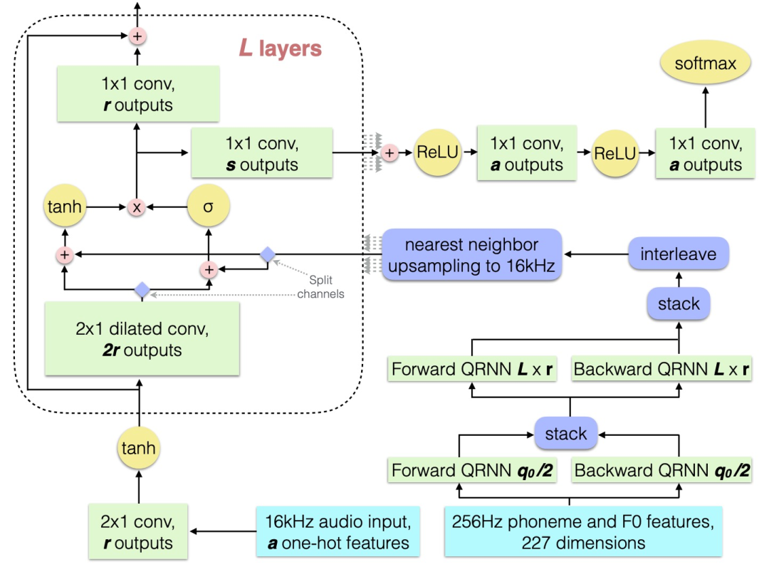
Figure 8. Modified WaveNet architecture. Each part is colored according to its function: brown for input, green for convolutions and QRNNs, yellow for unidirectional operations and softmax, pink for binary operations, and indigo for reshaping, transposing, and slicing.
| Model | SOTA! Platform Model Details Page |
|---|---|
| Deep Voice | Visit SOTA! Model Platform for implementation resources:https://sota.jiqizhixin.com/project/deep-voice |
Parallel WaveNet
Parallel WaveNet is a new method: probability density distillation. This method can produce high-fidelity speech samples at a speed 20 times faster than real-time, without significant differences in the quality of the generated speech, by training a parallel feedforward network using a trained WaveNet. It has now been able to provide multiple English and Japanese voices in production environments. In summary, Parallel WaveNet optimizes the basic WaveNet model in two ways to improve audio quality: first, by using 16-bit audio, the sampling model is replaced with a discretized mixture logistic distribution; second, by increasing the sampling rate from 16kHz to 24kHz, specific methods include increasing the number of layers, increasing the dilation factor, etc.
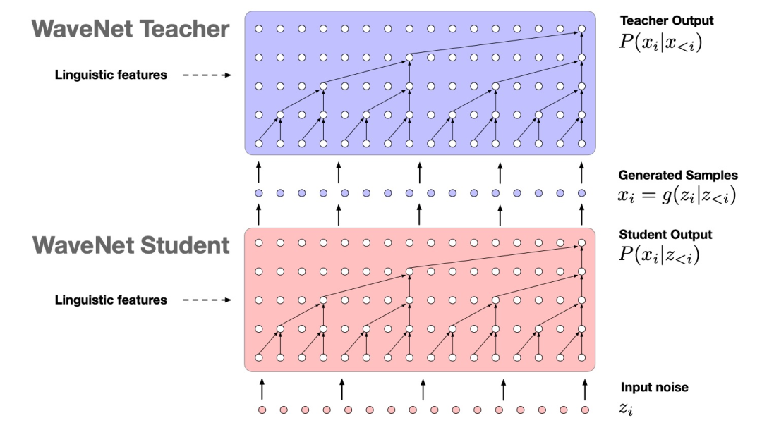
Figure 9. Overview of the probability density distillation method. A pre-trained WaveNet teacher is used to score the samples x output by the student. The student is trained to minimize the KL-divergence between its distribution and the teacher’s distribution, while maximizing the log likelihood of its samples under the teacher and simultaneously maximizing its own entropy.
Directly training the parallel WaveNet model with maximum likelihood is impractical because the inference process needed to estimate log likelihood is continuous and slow. Therefore, a new form of neural network distillation is introduced, using a pre-trained WaveNet as a “teacher” to effectively teach the “student” Parallel WaveNet. To emphasize the “standardized density model processing,” this process is termed probability density distillation (as opposed to probability density estimation). The basic idea is to have the student attempt to match the probability of its samples under the distribution learned by the teacher.
Given the parallel WaveNet student pS(x) and WaveNet teacher pT(x) trained on the audio dataset, the probability density distillation loss is defined as follows:

D_KL is the KL-divergence, H(P_S, P_T) is the cross-entropy between student P_S and teacher P_T, and H(P_S) is the entropy of the student distribution. When the KL divergence is zero, the student distribution perfectly recovers the teacher distribution. The entropy term (which was absent in previous distillation objectives) is critical because it prevents the student distribution from collapsing to the teacher mode. More importantly, all operations needed to estimate the derivatives of this loss (sampling from pS(x), evaluating pT(x), and evaluating H(pS)) can be performed efficiently.
The entropy term H(P_S) is expressed as:
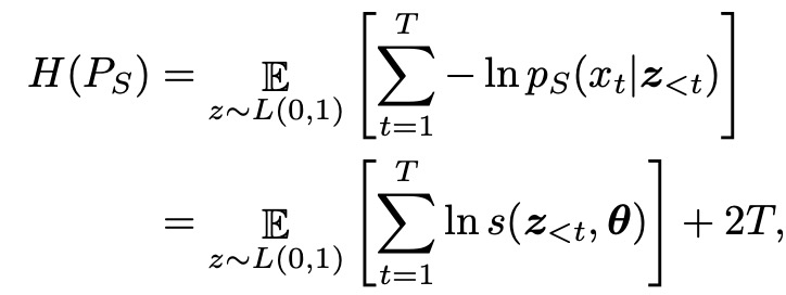
In the first equation, x = g(z), where z_t are independent samples derived from the logistic distribution. In the second equation, since the entropy of the logistic distribution L(u, s) is lns+2, we can compute this term without explicitly generating x. However, the cross-entropy term H(P_S, P_T) explicitly depends on x = g(z), and thus needs to be estimated by sampling from the student:
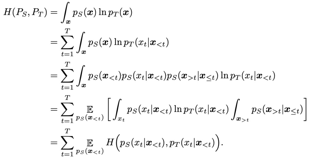
For each sample x drawn from the student pS, all pT(xt|x
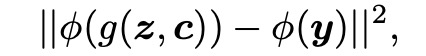
and contrastive distillation loss:

Currently, the SOTA! platform includes 2 model implementation resources for Parallel WaveNet.
| Item | SOTA! Platform Project Details Page |
|---|---|
| Parallel WaveNet | Visit SOTA! Model Platform for implementation resources:https://sota.jiqizhixin.com/project/parallel-wavenet |
GAN
This paper proposes a method for speech synthesis based on static parameters that combines generative adversarial networks, consisting of two neural networks: a discriminator that distinguishes between natural and generated samples, and a generator that deceives the discriminator. In the proposed framework, the discriminator is trained to distinguish between natural and generated speech parameters, while the acoustic model is trained to minimize the weighted sum of the traditional minimum generation loss and the adversarial loss used to deceive the discriminator. The goal of GAN is to minimize the KL-divergence between natural speech parameters and generated speech parameters, and the proposed method effectively mitigates the over-smoothing effect on the generated speech parameters. This paper considers both TTS and VC (Voice Conversion) tasks in experiments validating the effectiveness of the GAN model, where TTS is text-based speech synthesis, and VC is the technique for synthesizing speech with original language information from another speech (while preserving the original speech’s language information).
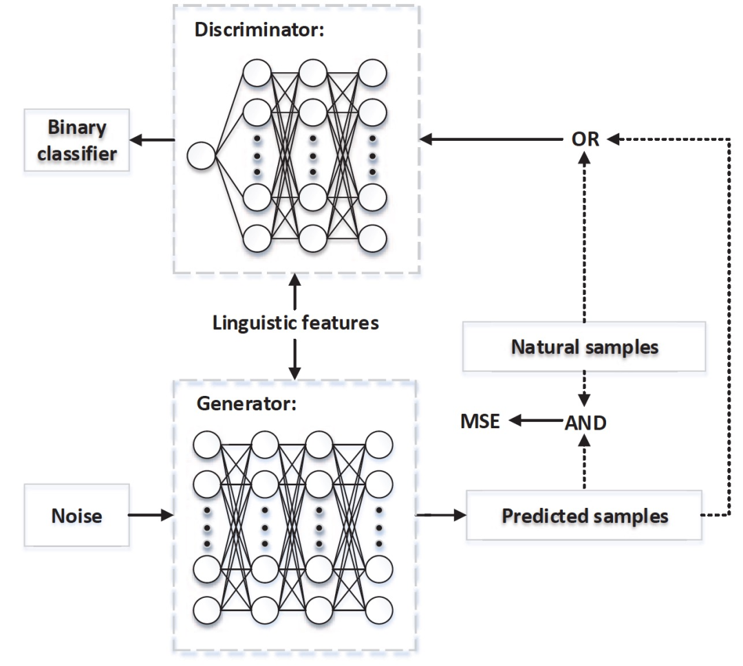
Figure 10. System schematic of the multi-task learning framework based on GAN
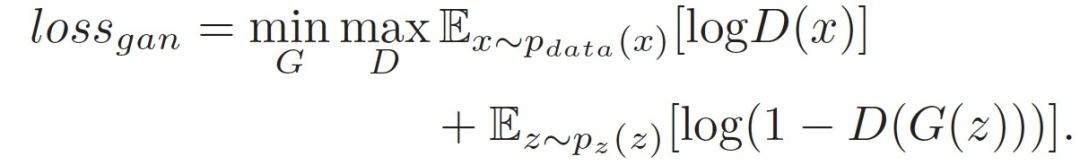
GAN is a generative model that learns the complex relationship between random noise input vectors z and output parameters y through an adversarial process. The estimation of GAN consists of two models: one is the generative model G, which captures the data distribution from random noise z; the other is the discriminative model D, which maximizes the probability of correctly distinguishing between real examples and fake samples generated from G. In this adversarial process, the generator tends to learn a mapping function G(z) to fit the real data distribution p_data(x) from a uniform random noise distribution p_z(z), while the discriminator aims to perfectly judge whether a sample comes from G(z) or p_data(x). Thus, both G and D are trained simultaneously in a two-player min-max game with a value function:
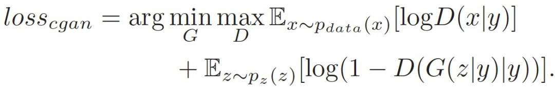
In the above generative model, due to weak guidance, the modes of generated samples cannot be controlled, thus introducing conditional generative adversarial networks (CGAN), which guide generation by considering additional information y. The loss function can be expressed as:
In traditional SPSS acoustic models, we usually minimize the MSE between the predicted parameters X_model and the natural speech X_real during the estimation process. This goal can be written as
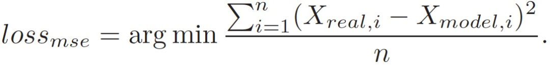
The numerical differences (in MSE) only involve estimation, and reducing numerical errors does not necessarily lead to perceived improvements in synthesized speech. To address this issue, GANs are introduced to learn the essential differences between synthesized and natural speech through the discriminative process. GANs can generate data rather than estimate density functions. To solve the model collapse problem in GANs, the following generator loss function is further proposed to guide GAN convergence to the optimal solution, allowing the generative model to produce expected data:
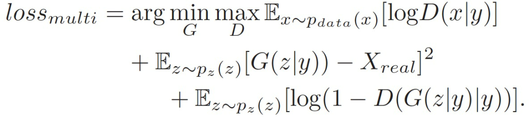
The final objective function is:

Considering language features as an additional vector y, and making input noise z follow a uniform distribution in the [-1,1] interval. Our framework can generate speech X_model through G(z|y), and during training, both loss_mse and loss_cgan are estimated simultaneously.
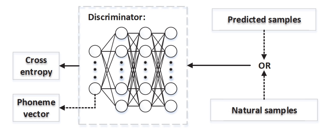
Figure 11. Discriminator with phoneme information
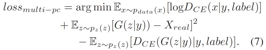
In the multi-task framework, attempts are made to use phoneme information to guide the discriminative process, as shown in Figure 11. Assuming the labels are a one-hot encoded vector representing phoneme categories, it is the category of the fake and real samples of D. Then our goal is to minimize the cross-entropy (CE) of the real samples while maximizing the loss of the fake samples, which means we do not know which phoneme the fake samples belong to. Therefore, the objective function of GANs can be updated to
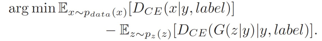
Considering phoneme classification, we arrive at the new loss function as follows:
Currently, the SOTA! platform includes 1 model implementation resource for GAN.
| Item | SOTA! Platform Project Details Page |
|---|---|
| GAN | Visit SOTA! Model Platform for implementation resources:https://sota.jiqizhixin.com/project/gan-voice |
Tacotron
Tacotron is an end-to-end TTS model that directly converts text to speech, consisting of an encoder, attention-based decoder, and a post-processing net. Similar end-to-end methods include WaveNet, DeepVoice, Char2Wav, etc. The structure of Tacotron is as follows:
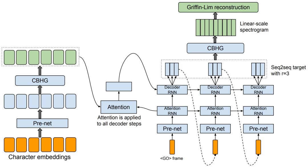
Figure 12. Model architecture. The model takes characters as input and outputs the corresponding raw spectrogram, which is then fed into the Griffin-Lim reconstruction algorithm to synthesize speech.
CBHG MODULE:
CBHG consists of a set of one-dimensional convolutional filters followed by highway networks and bidirectional gated recurrent units (GRUs). CBHG is a powerful module for extracting representations from sequences. The input sequence is first convolved with K groups of one-dimensional convolutional filters, where the k-th group contains Ck filters of width k (i.e., k=1,2,…,K). These filters explicitly model local and contextual information (similar to modeling single characters, bigrams, up to K-grams). The convolution outputs are stacked together and further maximally pooled along the time axis to increase local invariance. A stride of 1 can be used to preserve the original temporal resolution. The processed sequence is then passed to several fixed-width one-dimensional convolutions, whose outputs are added to the original input sequence through residual connections. Batch normalization is applied to all convolutional layers. The convolution outputs are sent to a multi-layer highway network to extract high-level features. Finally, a bidirectional GRU RNN is stacked on top to extract sequential features from both forward and backward contexts.
ENCODER:
The goal of the encoder is to extract a sequential representation of the text. The input to the encoder is a character sequence, where each character is represented as a one-hot vector and embedded into a continuous vector. A set of non-linear transformations, collectively referred to as “pre-net,” is then applied to each embedding. In this work, a bottleneck layer with dropout is used as the pre-net, which helps with convergence and improves generalization. A CBHG module transforms the output of the pre-net into the final encoder representation used by the attention module.
DECODER:
Using a content-based tanh Attention decoder, i.e., an additive model, an attention query is produced at each time step, concatenating the context vector and the output of the Attention RNN as the input to the decoder RNNs. The decoder RNNs use a stack of GRUs with longitudinal residual connections, generating outputs in the form of an 80-band mel-scale spectrogram through a simple fully connected layer, and then using a post-processing network to convert the seq2seq mel spectrogram into waveform.
POST-PROCESSING NET AND WAVEFORM SYNTHESIS:
The task of the post-processing network (post-processing net) is to convert the seq2seq target into a target that can be synthesized into a waveform. Since Griffin-Lim is used as the synthesizer, the post-processing network can learn to predict the spectral amplitudes sampled on a linear frequency scale. Furthermore, the post-processing network can obtain the complete decoding sequence. Unlike seq2seq, which always runs from left to right, it can utilize both forward and backward information to correct prediction errors for each individual frame. In this work, a CBHG module is used as the post-processing network. The concept of the post-processing network is highly general. It can be used to predict alternative targets, such as vocoder parameters, or as a neural vocoder similar to WaveNet to directly synthesize waveform samples. Finally, the Griffin-Lim algorithm is used for waveform synthesis.
Currently, the SOTA! platform includes Tacotron with 23 model implementation resources.
| Item | SOTA! Platform Project Details Page |
|---|---|
| Tacotron | Visit SOTA! Model Platform for implementation resources:https://sota.jiqizhixin.com/project/tacotron |
VoiceLoop
VoiceLoop is a neural text-to-speech (TTS) technology that converts text into speech from wild-sampled speech.
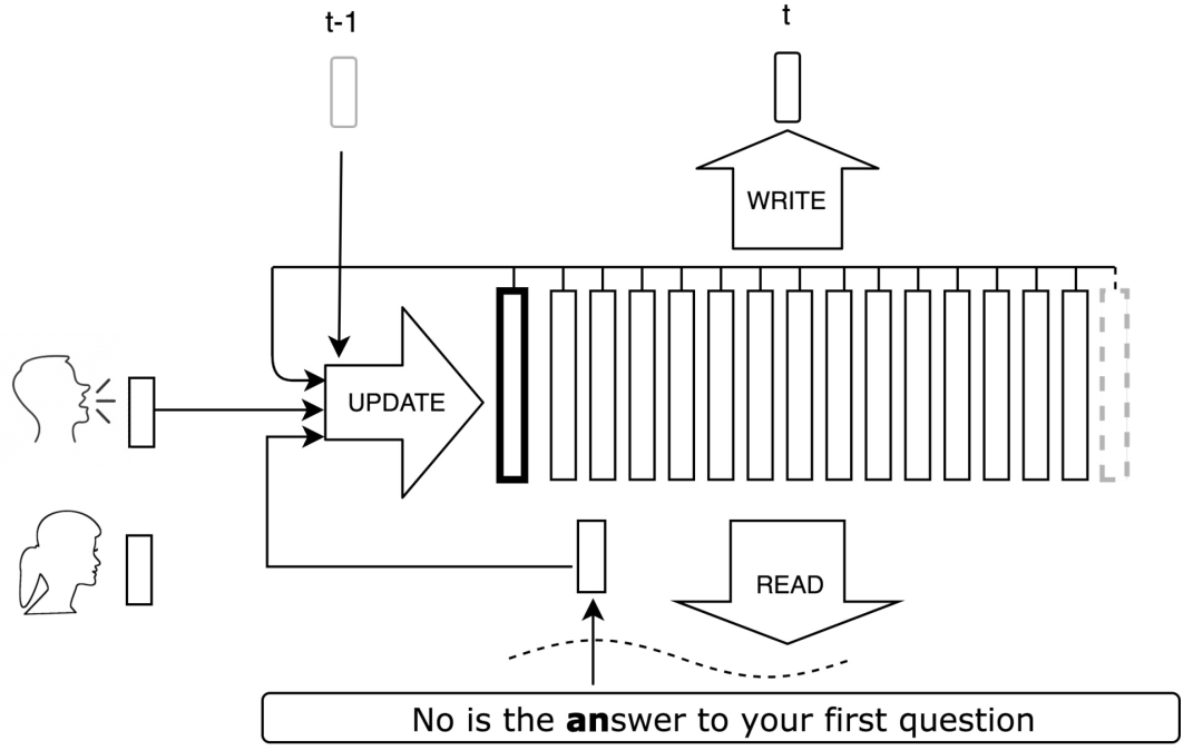
Figure 13. Overview of VoiceLoop architecture. The reader combines the phoneme encoding of the sentence with attention weights to create the current context. A new representation is created by a shallow network that takes context, speaker ID, previous output, and buffer as inputs. The new representation is inserted into the buffer, discarding the oldest vector in the buffer. The output is obtained by another shallow network that receives the buffer and speaker as inputs. Once training is complete, a new voice can be fitted by freezing the network, except for the speaker’s embedding.
VoiceLoop constructs a phonological store by implementing a shifting buffer as a matrix. Sentences are represented as lists of phonemes. A short vector is decoded from each phoneme. The current context vector is generated by weighting the phoneme encodings and summing them at each time point. The forward channel of the network operates in four sequential steps. After encoding the input sentence and speaker without context, the buffer plays a key role in all remaining steps, establishing connections between the components at each step. It also introduces error signals from the output back into the earlier steps.Step One: Encoding the Speaker and Input Sentence:
Each speaker is represented by a vector z. During training, the vectors of the speakers in training are stored in a lookup table LUT_s, which maps a running ID number to a representation of dimension d_s. For new speakers, i.e., speakers fitted after the network training, the vector z is calculated through a simple optimization process. Using CMU’s pronunciation dictionary, the input sentence is converted into a series of phonemes s1, s2, …, sl. The number of phonemes in the dictionary is 40, with two additional items added to represent different lengths of pauses. Each si is then mapped to an encoding based on a trained lookup table LUTp. This generates an encoding matrix E of size dp×l, where dp is the size of the encoding, and l is the sequence length.
Step Two: Calculating Context:
A monotonic attention mechanism based on Graves GMM is adopted. At each output time point t, the attention network N_a receives the buffer from the previous time step S_t-1 as input and outputs the GMM prior γt, shift κt, and logarithmic variation βt. For a GMM with c components, each component is a vector with a latent layer of dimension dk/10, and the activation function for the latent layer is ReLU.
Step Three: Updating the Buffer:
At each time step, a new representation vector u of dimension d is added to the first position St[1] of the buffer, discarding the last column of the previous time step St-1[k] in the buffer, while copying the rest to generate: St[i + 1] = St-1[i]. Step Four: Generating Output:
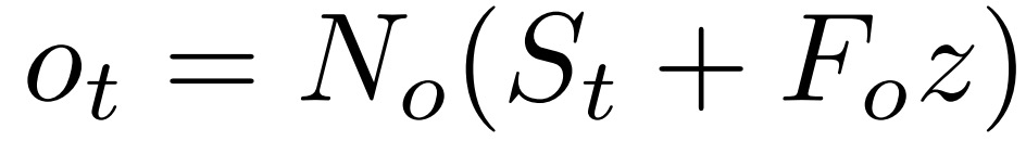
The output is generated using a network No with a structure similar to Na and Nu, along with a learned matrix Fo:
Significance of Memory Locations:
Using memory buffers instead of traditional RNNs shares memory across all processes and uses shallow, fully connected networks for all computations. To better understand the behavior of the buffer, consider the relative role of each buffer position. Specifically, the absolute values of weights from input (buffer elements) to the latent layer are averaged. The average is performed across all d features and dk/10 latent units, providing a value for each position.
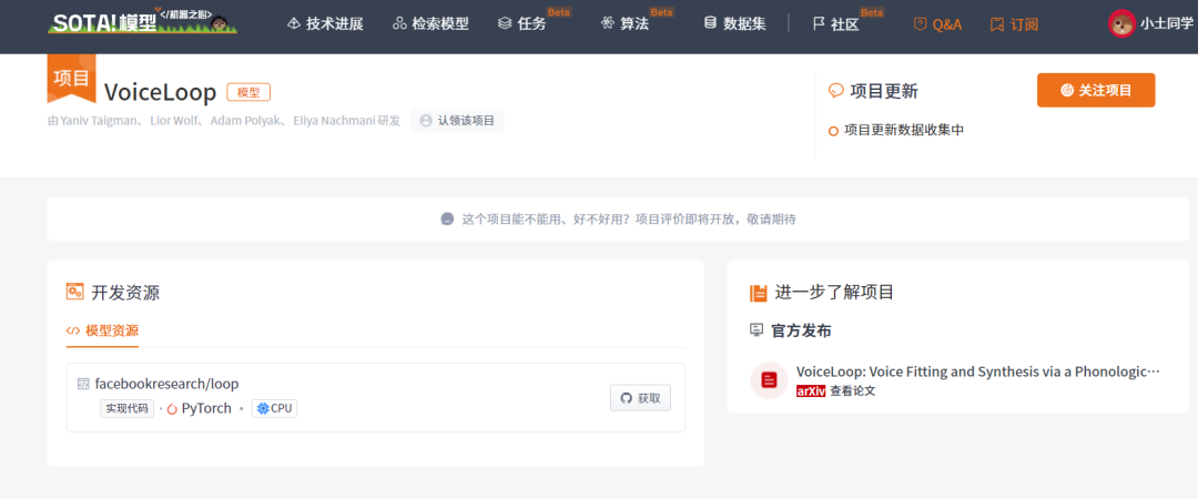
Currently, the SOTA! platform includes 1 model implementation resource for VoiceLoop.
| Model | SOTA! Platform Model Details Page |
|---|---|
| VoiceLoop | Visit SOTA! Model Platform for implementation resources:https://sota.jiqizhixin.com/project/voiceloop |
Visit SOTA! Model Resource Station (sota.jiqizhixin.com) to access the implementation code, pre-trained models, and APIs included in this article.
Web Access: Enter the new site address sota.jiqizhixin.com in the browser’s address bar to visit the “SOTA! Model” platform and check if the models you are interested in have new resources included.
Mobile Access: On the WeChat mobile end, search for the service account name “Machine Heart SOTA Model” or ID “sotaai”. Follow the SOTA! model service account to use the platform features through the bottom menu of the service account, with regular updates on the latest AI technologies, development resources, and community dynamics.