Summary of Basic Knowledge of Neural Networks

Click on the above “Beginner Learning Vision”, select to add Star or “Top”

Important content delivered immediately

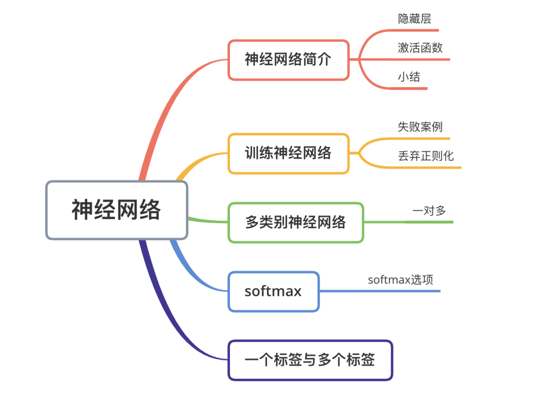
Overview of Structure

1. Introduction to Neural Networks

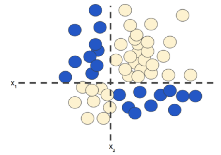
For nonlinear classification problems (as shown in Figure 1), “nonlinear” means that you cannot accurately predict labels using a model in the form of:

that is, the “decision surface” is not a straight line. Previously, we learned about a feasible method for modeling nonlinear problems – feature combinations.

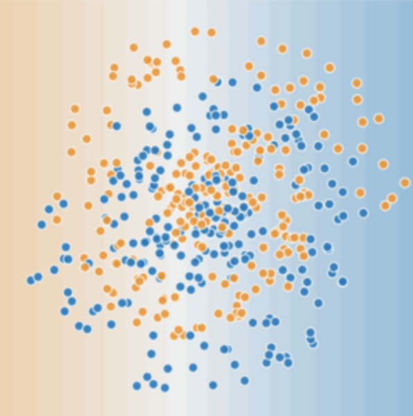
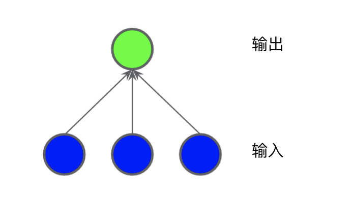
Now, please consider the following dataset

Figure 2. More Difficult Nonlinear Classification Problem

The dataset problem shown in Figure 2 cannot be solved with a linear model. To understand how neural networks can help solve nonlinear problems, we first present a linear model in a chart:

Figure 3. Linear Model Presented in a Chart

Each blue circle represents an input feature, and the green circle represents the weighted sum of the inputs. How can we change this model to improve its ability to handle nonlinear problems?

1.1 Hidden Layer

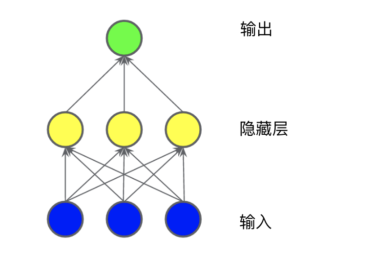
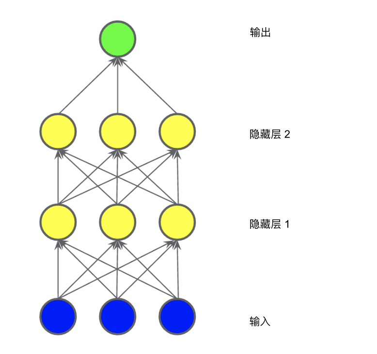
In the model shown in the diagram below, we added a “hidden layer” representing intermediate values. Each yellow node in the hidden layer is the weighted sum of the blue input node values. The output is the weighted sum of the yellow nodes.

Figure 4. Chart of Two-Layer Model

Is this model linear? Yes, its output is still a linear combination of its inputs.

In the model shown in the diagram below, we added another “hidden layer” representing the weighted sum.

Figure 5. Chart of Three-Layer Model

Is this model still linear? Yes, that’s correct. When you express the output as a function of the input and simplify it, you just get another weighted sum of the inputs, which cannot effectively model the nonlinear problem in Figure 2.

1.2 Activation Function

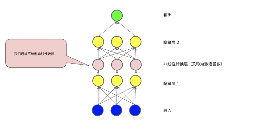
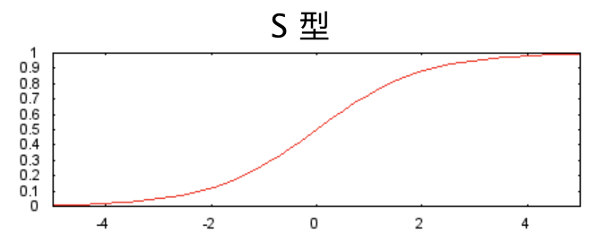
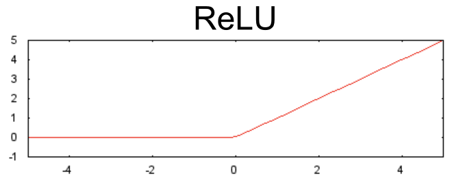
To model nonlinear problems, we can directly introduce nonlinear functions. We can connect each hidden layer node like a pipeline using nonlinear functions.

In the model shown in the diagram below, before the values of each node in hidden layer 1 are passed to the next layer for weighted summation, we apply a nonlinear function to transform them. This nonlinear function is called an activation function.

Figure 6. Chart of Three-Layer Model with Activation Function

Now that we have added an activation function, adding layers will have more impact. By stacking nonlinearities on top of nonlinearities, we can model extremely complex relationships between inputs and predicted outputs. In short, each layer can effectively learn more complex and higher-level functions through the original input. If you want a more intuitive understanding of how this process works, please refer to Chris Olah’s excellent blog post.

Common Activation Functions

The following S-shaped activation function converts the weighted sum into a value between 0 and 1.

The curve is as follows:

Figure 7. S-shaped Activation Function

Compared to smooth functions like the S-shaped function, the following rectified linear unit activation function (ReLU) typically performs better and is also very easy to compute.

The advantage of ReLU is that it has a more practical response range based on empirical findings (possibly driven by ReLU). The responsiveness of the S-shaped function decreases relatively quickly at both ends.

Figure 8. ReLU Activation Function

In fact, all mathematical functions can serve as activation functions. Assuming σσ represents our activation function (ReLU, S-shaped function, etc.), the value of the nodes in the network is specified by the following formula:

TensorFlow provides out-of-the-box support for various activation functions. However, we still recommend starting with ReLU.

1.3 Summary

Now, our model has all the standard components that people usually refer to as a “neural network”:

• A set of nodes, similar to neurons, located in layers.
• A set of weights representing the relationship between each neural network layer and the layer below it. The layer below may be another neural network layer or other types of layers.
• A set of biases, one for each node.
• An activation function that transforms the output of each node in the layer. Different layers may have different activation functions.

Warning: Neural networks do not always outperform feature combinations, but they can provide a flexible alternative suitable for many situations.

2. Training Neural Networks

This section discusses failure cases of the backpropagation algorithm and common methods for regularizing neural networks.

2.1 Failure Cases

Many common situations can lead to errors in the backpropagation algorithm.

Gradient Vanishing

The gradients of lower layers (closer to the input) can become very small. In deep networks, calculating these gradients may involve the product of many small terms.

As the gradients of lower layers gradually vanish to 0, the training speed of these layers becomes very slow, or they may stop training altogether.

The ReLU activation function helps prevent gradient vanishing.

Gradient Explosion

If the weights in the network are too large, the gradients of lower layers will involve the product of many large terms. In this case, the gradient will explode: the gradient becomes too large, making it difficult to converge. Batch normalization can reduce the learning rate, thus helping to prevent gradient explosion.

ReLU Unit Vanishing

Once the weighted sum of a ReLU unit falls below 0, the ReLU unit may stagnate. It outputs a 0 activation that contributes nothing to the network output, and the gradient cannot flow back through it during the backpropagation algorithm. With the source of the gradient cut off, the input to the ReLU may not be able to change sufficiently to bring the weighted sum back above 0.

Reducing the learning rate helps prevent ReLU unit vanishing.

2.2 Dropout Regularization

This is a form of regularization called dropout that can be used in neural networks. It works by randomly dropping some network units at each step of the gradient descent method. The more you drop, the stronger the regularization effect:

• 0.0 = No dropout regularization.
• 1.0 = Drop everything. The model learns nothing.

Values between 0.0 and 1.0 are more useful.

3. Multi-class Neural Networks

3.1 One-vs-All

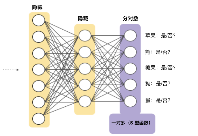
One-vs-all provides a method to utilize binary classification. Given that a classification problem may have N feasible solutions, the one-vs-all solution includes N separate binary classifiers, each corresponding to a possible outcome. During training, the model trains a series of binary classifiers, each answering a separate classification problem. For example, in the case of a dog photo, it may need to train five different classifiers, where four will treat the image as a negative sample (not a dog), and one will treat the image as a positive sample (is a dog). That is:

1. Is this an image of an apple? No.
2. Is this an image of a bear? No.
3. Is this an image of candy? No.
4. Is this an image of a dog? Yes.
5. Is this an image of an egg? No.

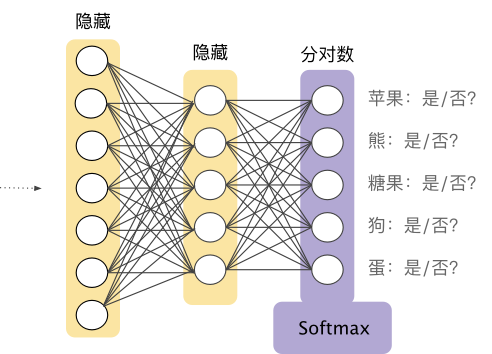
This method is reasonable when the total number of categories is small, but as the number of categories increases, its efficiency becomes increasingly low.

We can create a significantly more efficient one-vs-all model using deep neural networks (where each output node represents a different category). Figure 9 illustrates this method:

Figure 9. One-vs-All Neural Network

4. Softmax

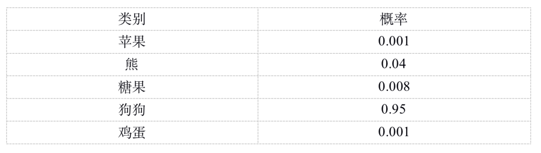
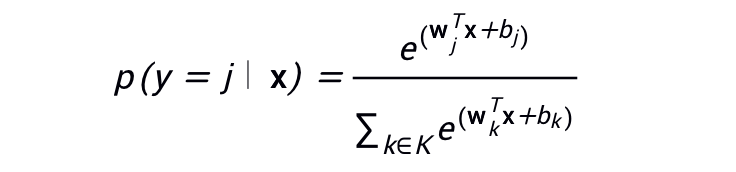
We already know that logistic regression can produce decimals between 0 and 1. For example, a logistic regression output value of 0.8 for an email classifier indicates an 80% probability that the email is spam and a 20% probability that it is not spam. Clearly, the sum of the probabilities of an email being spam or not spam equals 1.0.

Softmax extends this idea to the multi-class domain. That is, in multi-class problems, Softmax assigns a probability represented as a decimal to each category. The sum of these probabilities must equal 1.0. This additional constraint helps the training process converge more quickly compared to other methods.

For example, returning to the image analysis example we saw in Figure 9, Softmax might yield the following probabilities for the image belonging to a specific category:

The Softmax layer is the neural network layer immediately before the output layer. The Softmax layer must have the same number of nodes as the output layer.

Figure 10. Softmax Layer in Neural Networks

The Softmax equation is as follows:

Please note that this formula essentially extends the logistic regression formula to multiple categories.

4.1 Softmax Variants

Please check the following Softmax variants:

• Complete Softmax is the Softmax we have been discussing; that is, Softmax calculates probabilities for each possible category.
• Candidate Sampling refers to Softmax calculating probabilities for all positive category labels but only calculating probabilities for random samples of negative category labels. For example, if we want to determine whether an input image is a picture of a Beagle or a Bloodhound, we do not need to provide probabilities for every non-dog sample.

Complete Softmax incurs low costs when the number of categories is small, but as the number of categories increases, its cost becomes extremely high. Candidate sampling can improve efficiency when dealing with problems with a large number of categories.

5. Single Label vs. Multi-label

Softmax assumes that each sample is a member of only one category. However, some samples can belong to multiple categories simultaneously. For such examples:

• You cannot use Softmax.
• You must rely on multiple logistic regressions.

For example, suppose your sample is a picture containing only one item (a piece of fruit). Softmax can determine the probability that the item is a pear, orange, apple, etc. If your sample is a picture containing a variety of items (a few different types of fruits), you must switch to multiple logistic regressions.

Download 1: OpenCV-Contrib Extension Module Chinese Version Tutorial

Reply "Extension Module Chinese Tutorial" in the backend of the "Beginner Learning Vision" public account to download the first OpenCV extension module tutorial in Chinese, covering installation of extension modules, SFM algorithms, stereo vision, object tracking, biological vision, super-resolution processing, and more than twenty chapters of content.

Download 2: Python Vision Practical Project 52 Lectures

Reply "Python Vision Practical Project" in the backend of the "Beginner Learning Vision" public account to download 31 visual practical projects including image segmentation, mask detection, lane line detection, vehicle counting, adding eyeliner, license plate recognition, character recognition, emotion detection, text content extraction, facial recognition, etc., to help quickly learn computer vision.

Download 3: OpenCV Practical Project 20 Lectures

Reply "OpenCV Practical Project 20 Lectures" in the backend of the "Beginner Learning Vision" public account to download 20 practical projects based on OpenCV for advanced learning of OpenCV.

Group Chat

Welcome to join the reader group of the public account to communicate with peers. Currently, there are WeChat groups for SLAM, 3D vision, sensors, autonomous driving, computational photography, detection, segmentation, recognition, medical imaging, GAN, algorithm competitions, etc. (will gradually be subdivided in the future). Please scan the WeChat number below to join the group, and note: "Nickname + School/Company + Research Direction", for example: "Zhang San + Shanghai Jiao Tong University + Vision SLAM". Please follow the format; otherwise, you will not be approved. After successful addition, you will be invited to the relevant WeChat group based on your research direction. Please do not send advertisements in the group; otherwise, you will be removed from the group. Thank you for your understanding~