

Big Data Digest Work
Compiled by: Xiao Fan Pen, Zhou Jiayu, Da Jieqiong, Qian Tianpei
Douban Water Army Detection, “Game of Thrones” Sequel, and the Ever-More Amazing Google Translate…
Recently, various applications of Natural Language Processing (NLP) have been thriving.
These NLP applications seem to be incredibly cool, but the principles behind them are not difficult to understand.
Today, we will explore the most commonly used natural language processing techniques and models, guiding you step by step to create a simple and amazing little application.
No exaggeration, 90% of NLP problems can be solved using similar methods.
This tutorial teaches you natural language processing from the three major stages of data processing:
-
Collecting, preparing, and checking data
-
Building simple models (including deep learning models)
-
Interpreting and understanding your model
The entire tutorial’s Python code is available here:
https://github.com/hundredblocks/concrete_NLP_tutorial/blob/master/NLP_notebook.ipynb
Let’s get started!
Step 1: Collecting Data
There are numerous sources for natural language data! Taobao reviews, Weibo, Baidu Encyclopedia, etc.
However, today we will process a dataset from Twitter called the “Disasters on Social Media” dataset.
We will use a dataset generously provided by CrowdFlower, which consists of over ten thousand tweets related to disasters.
Some of these tweets indeed describe disaster events, while the rest are movie reviews, jokes, and other strange things.
Our task will be to detect which tweets are about a disastrous event and which ones are irrelevant topics, such as movies. Why do this? Relevant departments can use this small application to obtain timely disaster event information!
Next, we will refer to tweets related to disasters as “disaster” and others as “irrelevant”.
Labels
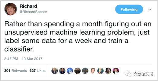
Note that we are using labeled data. As NLP expert Socher said, instead of spending a month using unsupervised learning to process a bunch of unlabeled data, it is better to spend a week labeling some data and create a classifier.
Step 2: Cleaning Data
The first principle we follow is: “No model can save bad data.” So, let’s clean the data first!
We will perform the following operations:
1. Remove all irrelevant characters, such as any non-alphanumeric characters
2. Tokenize your text into individual words
3. Remove irrelevant words, such as “@” mentions or URLs
4. Convert all characters to lowercase so that words like “hello”, “Hello”, and “HELLO” are treated as the same word
5. Consider consolidating misspelled or differently spelled words into one representation (e.g., combining “cool”, “kewl”, “cooool”)
6. Consider lemmatization (reducing words like “am”, “are”, “is” to a common form like “be”)
After following these steps and checking for other errors, we can start training our model with the clean tokenized data!
Step 3: Finding a Good Data Representation
After cleaning the data, we still need to convert this text into numbers—so that machines can understand it!
For example, in image processing, we need to convert images into a matrix representing pixel RGB intensity values.

A smiley face represents a numerical matrix
Representations in natural language processing are slightly more complex. We will try various representation methods.
One-Hot Encoding (Bag of Words)
A natural way to represent text for computers is to individually encode each character as a number (e.g., ASCII).
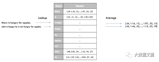
For example, we can build a vocabulary of all unique words in the dataset and associate a unique index with each word in the vocabulary. Then, each sentence is represented as a list of the same length as the number of unique words in our vocabulary. At each index in this list, we mark the occurrence of the given word in our sentence. This is called a bag-of-words model because it completely ignores the order of words in our sentences, as shown below.
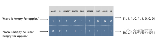
Representing sentences as a bag of words. On the left is the sentence, and on the right is its representation. Each index in the vector represents a specific word
Visualizing Embeddings
In the “Disasters on Social Media” example, we have about 20,000 unique words, which means each sentence will be represented as a vector of length 20,000. This vector will contain mostly zeros since each sentence contains only a small subset of our vocabulary.
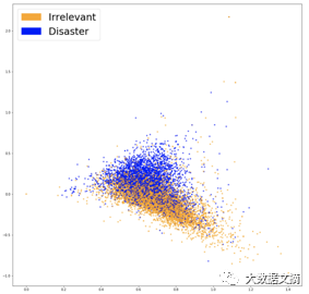
To understand whether our representation captures information related to our problem (i.e., whether tweets are related to disasters), it is a good idea to visualize them and see if these classes seem well-separated. Since vocabularies are usually very large and it is impossible to display data in 20,000 dimensions, techniques like PCA will help project the data into two dimensions, as shown:
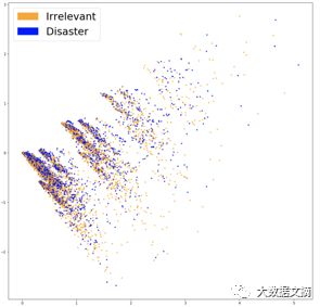
Visualization
These two classes do not seem well-separated, which could be a feature of our embeddings or merely due to dimensionality reduction. To see if the bag-of-words features are useful, we can train a classifier based on them.
Step 4: Classification
When first encountering a problem, a general best practice is to start with the simplest tools. Whenever it comes to classifying data, a common preference for generality and interpretability is Logistic Regression. It is very easy to train, and the results can be interpreted because you can easily extract the most important coefficients from the model.
We will split the data into a training set for fitting the model and a test set for evaluating the model’s generalization ability to unseen data. After training, we achieved an accuracy of 75.4%. Not bad! If we simply guessed the most frequent class (“irrelevant”), the accuracy would only reach 57%. However, even though 75% accuracy is sufficient for our needs, we should not release a model without trying to understand it.
Step 5: Evaluation
Confusion Matrix
The first step is to understand the types of errors our model makes and which types of errors are most undesirable. In our case, false positives classify as irrelevant when they are actually disasters, while false negatives classify as disasters when they are labeled as irrelevant. If we want to prioritize every potential event, we would want to reduce our false negatives. However, if we are resource-constrained, we may prioritize reducing false positives to decrease false alarms. A good way to visualize this information is to use a confusion matrix, which compares our model’s predictions to the true labels. Ideally, the matrix would show a diagonal line from the top left corner to the bottom right (perfect match of predictions and actual).
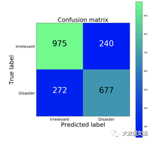
Confusion matrix (green is high, blue is low)
Relative to false positives, our classifier produces more false negatives proportionally. In other words, the most common mistake our model makes is classifying disasters as irrelevant. If false positives result in high enforcement costs, this gives our classifier a good bias.
Model Interpretation
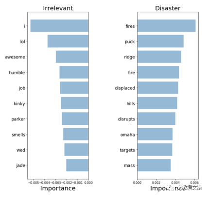
To validate our model and analyze its prediction accuracy, it is crucial to see which words it uses to make decisions. If our data is biased, then the classifier will only make accurate predictions on the sample data, and this model may not generalize well in the real world. Here, we plot the “most critical words” table for both disaster and irrelevant. Since we can extract and rank the coefficients used for prediction in the model, it is quite simple to calculate the importance of words using bag-of-words and logistic regression.
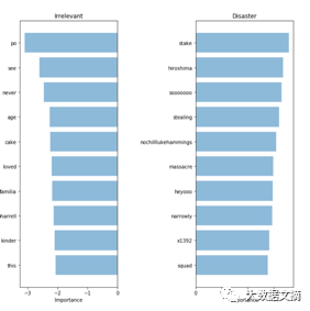
Bag of words: keywords
Our classifier correctly identified some patterns (like Hiroshima and massacre), but there are also clearly some seemingly meaningless overfitting (like heyoo blues rock and x1392 topic abbreviation). Now, our bag-of-words model is handling a huge vocabulary containing various different words and treating all words equally. However, some of these words appear very frequently and only affect our predictions. Next, we will try a new method to represent sentences that can statistically account for word frequency to see if we can extract more signal from our data.
Step 6: Statistical Vocabulary Structure
To make our model focus more on meaningful words, we can use TF-IDF scoring (Term Frequency-Inverse Document Frequency) on top of the bag-of-words model. TF-IDF determines the weight of a word based on its occurrence frequency in the dataset, reducing the weight of overly frequent words while increasing its relevance against noise interference. The following image shows the PCA projection of our newly embedded data.
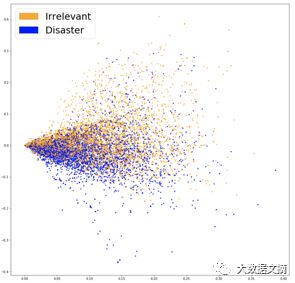
TF-IDF embedding visualization
From the above image, there is a relatively clear boundary between the two colors. This will make it easier for our classifier to separate them into two groups. Let’s see if this leads to better performance! Next, we will train another logistic regression model on our new embedded data, achieving an accuracy of 76.2%.
This is a very subtle improvement. Has our model started to adopt more critical words? If we achieve better results while preventing our model from “cheating”, then we can truly consider this model a breakthrough.
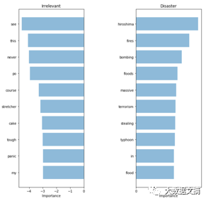
TF-IDF: keywords
The words that the model takes appear to be more relevant! Although the metrics on our test set only show a slight increase, we will have more confidence in the terms used by the model, making it more comfortable to apply in systems interacting with customers.
Step 7: Cleverly Utilizing Semantics
Turning Words into Vectors
Our latest model manages to use high-signal words. However, if we configure this model, we will likely encounter words that we have not seen in the training set before. However, even when training, similar words may not be accurately distinguished by previous models.
To solve this problem, we need to capture the semantics of words, meaning we need to understand that words like “good” and “positive” are closer than “apricot” and “continent”. We will use a tool called Word2Vec to help us capture semantics.
Using Pre-trained Words
Word2Vec is a technique for implementing continuous word embeddings. It learns by reading large amounts of text and remembers which words tend to appear in similar contexts. After training on enough data, it generates a 300-dimensional vector for each word in the vocabulary, with semantically similar words being closer together.
The author of this article has open-sourced a model that is pre-trained on a very large corpus, allowing us to incorporate some semantic knowledge into our model. Pre-trained vectors can be found in the knowledge base related to this article.
Sentence-Level Representation
A quick way to obtain sentence embeddings for our classifier is to average the Word2Vec scores of all words in the sentence. This is similar to the bag-of-words approach, but this time we discard the grammar of the sentence while retaining some semantic information.
Word2Vec Sentence Embedding
The following image visualizes the new embeddings obtained using previous techniques:
Word2Vec Embedding Visualization
The boundary between the two color groups appears more distinct, and our new embedding technique is likely to help our classifier find separation between the two classes. After training the same model again (using logistic regression), we achieved an accuracy of 77.7%, which is the best result we have obtained so far! Next, we should check our model.
Complexity vs. Interpretability Trade-off
Since the new embedding technique does not represent each word as a one-dimensional vector like our previous models, it is difficult to see which words are most relevant to our classification. While we can still use the coefficients of logistic regression, they only correlate with our 300-dimensional embedding rather than the vocabulary index.
For such a low accuracy, losing all interpretability seems to be a tough trade-off. However, for more complex models, we can utilize black-box interpreters like LIME to gain insights into how the classifier works.
Github provides LIME through open-source packages. The black-box interpreter allows users to explain any classifier’s decisions by perturbing the input (in our case, removing words from sentences) and observing changes in predictions.
Next, let’s examine a few sentences from our dataset for interpretation.
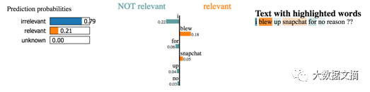
However, we do not have time to explore the thousands of cases in the dataset. What we should do is continue running LIME on typical examples of test cases to see which words remain prominent. Through this method, we can obtain the importance scores of words like our previous models and validate the predictions of the model.

Word2Vec: keywords
The model seems to be able to extract highly relevant words, suggesting that it can make understandable decisions. These appear to be the most relevant words among all previous models, so we are more willing to deploy it in practical operations.
Step 8: Cleverly Utilizing Semantics with an End-to-End Approach
We have introduced fast and effective methods to generate compact sentence embeddings. However, by omitting word order, we lose all syntactic information of the sentence. If these methods do not provide sufficient conclusions, more complex models can be used to take the entire sentence as input and predict labels without building intermediate representations. A common approach is to treat sentences as a sequence of word vectors, using Word2Vec or newer methods like GloVe or CoVe. This is what we will do next.
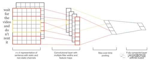
Efficient end-to-end architecture (source)
Training convolutional neural networks for sentence classification is very fast, and as an entry-level deep learning architecture, it performs well. Although convolutional neural networks (CNNs) are primarily known for their performance on image data, they have long provided excellent results on text-related tasks and typically train faster than most complex NLP methods (like LSTM and encoder/decoder architectures). This model retains word order and learns valuable information about which word sequences can predict our target class. Unlike previous models, it can distinguish between “Alex eats plants” and “plants eat Alex”.
Training this model does not require more work than previous methods (see code), and it gives us a better model than before, achieving an accuracy of 79.5%! Like the models mentioned above, the next step should be to continue exploring and interpreting predictions to verify it is indeed the best model configured for users. Now, you should be able to tackle this problem on your own.
Summary
-
Start with a simple and quick model
-
Interpret its predictions
-
Understand the types of errors it makes
-
Use this knowledge to determine the next steps: whether the model is effective for the data or if a more complex model should be used
These methods are applied to specific cases, such as understanding and utilizing short text models like tweets, but in reality, these ideas are broadly applicable to various problems!
As mentioned at the beginning, 90% of natural language processing problems can be solved using this approach, which is as easy as cutting vegetables!
Original link:
[Today’s Machine Learning Concept]
Have a Great Definition
Volunteer Introduction