
This article is a translated version of the notes from Stanford University’s CS224d course, authorized by Professor Richard Socher of Stanford University. Unauthorized reproduction is prohibited; for specific reproduction requirements, please see the end of the article.
Translation: Hu Yang & Xu Ke
Proofreading: Han Xiaoyang & Long Xincheng
Editor’s Note: This article is the seventh installment of our series on the Stanford University CS224d Course. The content covers the RNN, LSTM, and GRU sections of Stanford’s CS224d course for interested readers to experience and learn.
Additionally, for readers interested in further study and communication, we will organize learning exchanges through QQ groups (due to the limitations of WeChat group sizes).
Long press the following QR code to directly join the QQ group
Or join the group with number 564538990

◆ ◆ ◆
1. Language Model
A language model is used to calculate the probability of a specific sequence of words occurring. The joint probability of a vocabulary sequence of length m  is represented as
 Since we know the number of words before obtaining specific vocabulary, the properties of the vocabulary
  change based on their position in the input document, and the calculation of the joint probability
  typically only considers a window of words that contains prefix words instead of all prefix words:
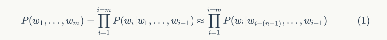
Formula 1 plays a crucial role in determining whether a sequence of words corresponds to the correct generated result for a given input sequence in speech recognition and machine translation systems. In a given machine translation system, for each translation task of phrases or sentences, the software is usually required to generate a set of alternative word sequences (e.g., “I have already”; “I used to have”; “I have”; “I have already”; “I possess”) along with their scores to determine whether they can form the optimal translation sequence.
In machine translation tasks, the model finds the best answer word sequence for the input phrase by measuring and comparing the scores of various alternative output word sequences. To accomplish this, the model needs to frequently switch between two task models: word ordering and word selection. The aforementioned goal will be achieved by setting up a probability calculation function for all candidate word sequences that compares the scores of these candidate word sequences. The candidate word sequence with the highest score is the output of the machine translation task.
For example: In the comparative sentence “This small cat is really”, the machine gives a higher score to the example sentence “This cat is really small” compared to “Walking to the house after school”, where “Walking home after school” will receive a higher score. To calculate these probabilities, the effects of statistical n-gram language models and word frequency models will be compared. For instance, if a bigram language model is chosen, the frequency of semantic bigrams is calculated by counting the current word and its preceding word, which needs to be distinguished from the frequency calculation method of a unigram model. Formulas 2 and 3 show how the bigram semantic model and trigram semantic model handle this relationship.

The relationship expressed in Formula 3 focuses on predicting subsequent words based on the fixed window content in the context (e.g., the range of n prefix words). In some cases, merely extracting n prefix words as the window range may not adequately capture contextual information. For example, when an article emphasizes the history between Spain and France in the later sections, if you read the sentence “These two countries are heading toward war” in the earlier text, just having the preceding text of this sentence clearly does not allow us to identify the named entities of these two countries. Bengio et al. proposed the first large-scale deep learning natural language processing framework, which can capture the aforementioned contextual relationships by learning to obtain distributed representations of vocabulary.
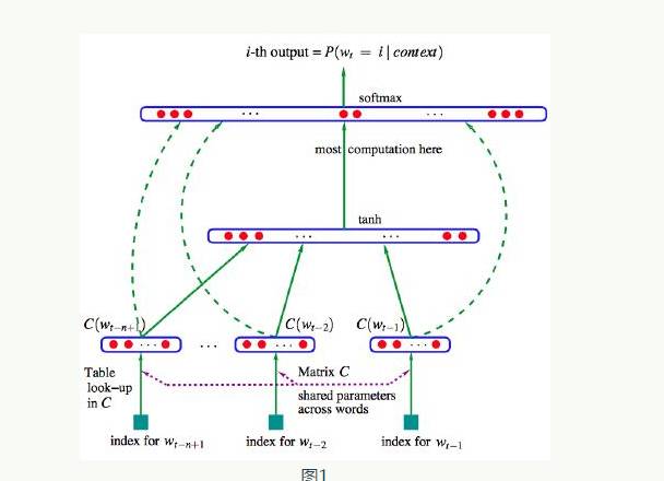
Figure 1 illustrates the framework of this neural network. In this model, input word vectors are utilized in both the hidden layer and output layer. Formula 4 displays the parameters in the softmax() classification function that incorporates the standard tanh() function, which acts as a linear classifier,  represents the input word vectors of all prefix words.

However, in all traditional language models, the scale of language memory information containing n-length windows grows exponentially with the operation of the system, so facing large word windows, if the memory information is not extracted and processed separately, the above task is almost impossible to accomplish.
◆ ◆ ◆
2. Recurrent Neural Networks (RNN)
Unlike traditional machine translation models that only consider limited prefix vocabulary information as conditional items for semantic models, recurrent neural networks (RNN) have the capability to incorporate all preceding vocabulary from the corpus into the model’s considerations.
Figure 2 shows the architecture of the RNN model, where each vertical rectangle represents the hidden layer for each iteration, t. Each such hidden layer has several neurons, each performing linear matrix operations on the input vector and outputting results through nonlinear operations (e.g., the tanh() function). In each iteration, the output from the previous iteration changes with the next word’s word vector in the document, , which is the input to the hidden layer, and the hidden layer will produce predicted output values
 and provide the output feature vector to the next hidden layer
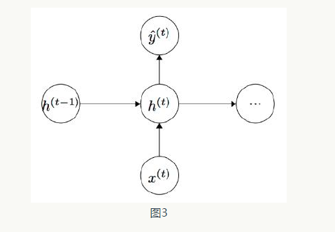
 (see formulas 5 and 6). The input and output conditions of each individual neuron are shown in Figure 3.
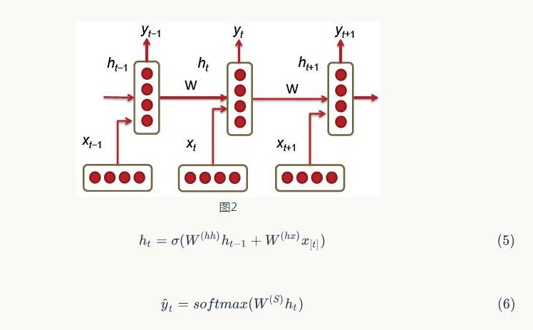
The details and meanings of the parameter settings in the network are as follows:
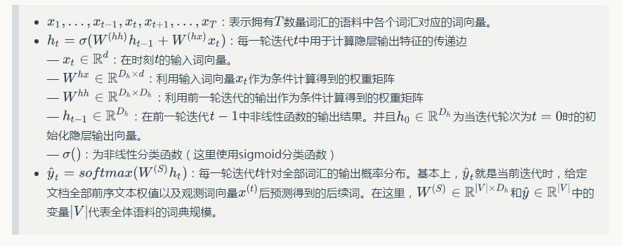
In recurrent neural networks, the loss function is usually set as the previously mentioned cross-entropy error rate. Formula 7 shows the summation of this function over the entire vocabulary at iteration t.

On a corpus of size T, the cross-entropy error rate is calculated as follows:
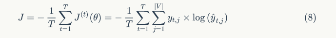
Formula 9 is used to represent the perplexity relationship; its calculation is based on the exponent of 2, with the exponent being the negative logarithm of the cross-entropy error rate function shown in Formula 8. Perplexity is used to measure the degree of disturbance of a low-value function when considering more conditional items during subsequent word prediction (compared to the actual results).

The memory required to execute one layer of the RNN network is proportional to the number of words in the corpus. For example, a sentence with k words will occupy the space of k word vectors in memory. Additionally, the RNN network will maintain two pairs of W and b matrices. Although the size of matrix W may be very large, its size does not change with the scale of the corpus (unlike traditional models). For an RNN network iterated for 1000 rounds, W will be a 1000X1000 matrix and is independent of the corpus size.
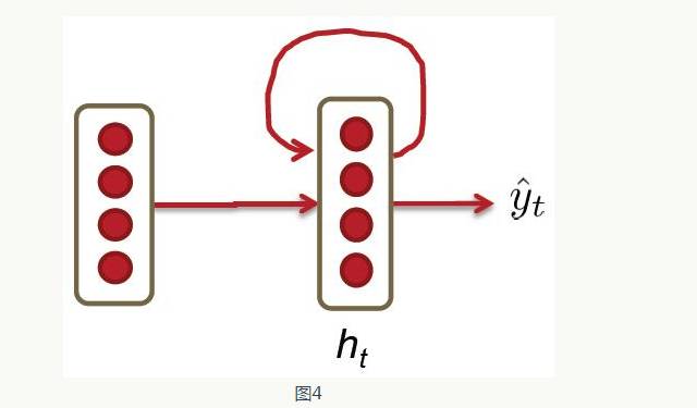
Figure 4 shows another representation of the RNN neural network model from some publications. It represents each hidden layer of the RNN neural network as a ring.
2.1 Gradient Vanishing and Exploding Problems
From the sequential steps, we can derive the propagation weight matrix in the recurrent neural network; the RNN model ensures that the goal is to propagate content information through multiple iterative steps. The following two sentences can help deepen the understanding:
Sentence 1: “Jane walked into the room. John also walked into the room. Jane said hello to ___”
Sentence 2: “Jane walked into the room. John also walked into the room. Because it was getting late, people went home after working all day. Jane said hello to ___”
In the above two examples, based on the context, most of the time we know the answer in the blank is “John”. The relative word distance of the second person appearing in the context is very important for the RNN model to predict the next word as “John”. From our understanding of RNNs, theoretically, this part needs to be given. However, experiments show that the prediction accuracy of the blank in sentence 1 is higher than that in sentence 2. This is because during the backpropagation phase, the gradient contribution value gradually decreases in the early propagation steps. Therefore, for long sentences, the longer the content, the lower the probability of identifying “John” as the word in the blank. We will later discuss the mathematical reasoning behind the gradient vanishing problem.
In a given iteration t, considering formulas 5 and 6, used to calculate the RNN error rate  we calculate the total error rate for each step of iteration. Thus, the error rate
  for each step t can be calculated from the previously listed calculations.

By applying the chain rule to the results of formulas 5 and 6, we obtain the error rate for each iterative step. Equation 11 shows the corresponding derivation process.  represents the partial derivative of the previous k iterations.
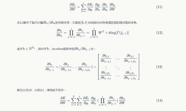
Formula 15 is the norm of the Jacobian matrix of equation 13. Where  represents the upper boundary of the norms of the two matrices. According to formula 15, we calculate the partial gradient norms at each iteration t.
 using
using norms to calculate the norms of the above two matrices. For a given sigmoid non-linear function, the norm
 can only be 1.


During the experiments, once the gradient value grows too large, it can easily lead to overflow (such as: infinity and non-numeric values); this is the gradient explosion problem. However, when the gradient value approaches zero, for words that are far apart in the corpus, it greatly reduces the learning quality of the model, and the gradient will continue to decay; this is the gradient vanishing problem.
If you want to understand the practical issues of the gradient vanishing problem, you can visit the example website below.
2.2 Solutions to Gradient Explosion and Vanishing
The above text introduced some situations of gradient vanishing and exploding in deep neural networks; we now begin to attempt to address these issues with some heuristic methods.
To solve the gradient explosion problem, Thomas Mikolov first proposed a simple heuristic solution, which is to truncate the gradient to a smaller number when it exceeds a certain threshold. Specifically described in Algorithm 1:
Algorithm 1: Truncate Gradient When Gradient Explodes (Pseudocode)
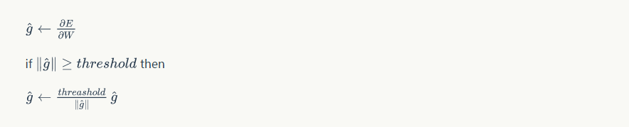
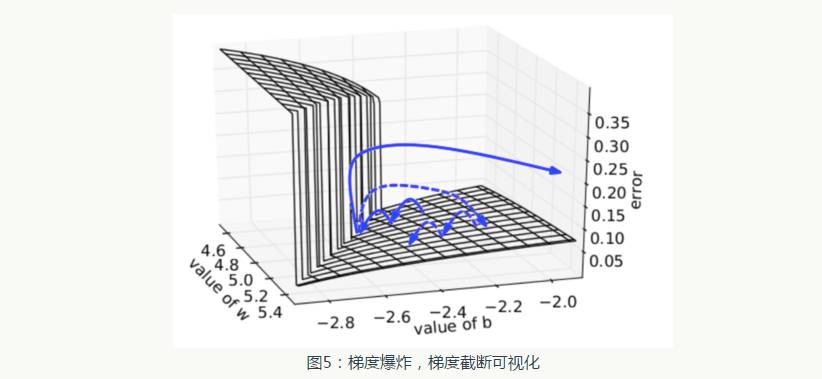
Figure 5 visualizes the effect of gradient truncation. It shows a small RNN (where W is the weight matrix and b is the bias term) decision surface. This model consists of a small segment of RNN units; solid arrows indicate the training process of gradient descent at each step. When the gradient descent process encounters a high error in the model’s objective function, the gradient is sent away from the decision surface. The truncated model creates a dashed line that pulls the error gradient back to a position close to the original gradient.
 To address the gradient vanishing problem, we introduce two methods. The first method is to change random initialization
 to a related matrix initialization. The second method is to use ReLU (Rectified Linear Units) instead of the sigmoid function. The derivative of ReLU is either 0 or 1. Thus, the gradient of the neurons will always be 1, and it will not decrease after propagating for a certain time.
2.3 Deep Bidirectional RNNs
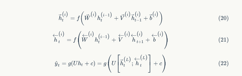
As previously mentioned, in a word sequence, we utilize RNN technology and past words to predict the next word. Similarly, we can also predict based on future words. Irsoy et al. designed a bidirectional deep neural network, where at each time node t, this network has two layers of neurons, one layer propagating from left to right and the other from right to left. To ensure that there are two hidden layers at any moment t, this network needs to consume double the storage to store parameters such as weights and biases. The final classification result is produced by combining the two layers of RNN hidden layers. Figure 6 shows the structure of the bidirectional network, and formulas 17 and 18 represent the mathematical meaning of the bidirectional RNN hidden layers. The only difference in these two relationships is the direction of the cycle. Formula 19 shows how to predict the next word by summarizing the representations of past and future words using the category relationships.
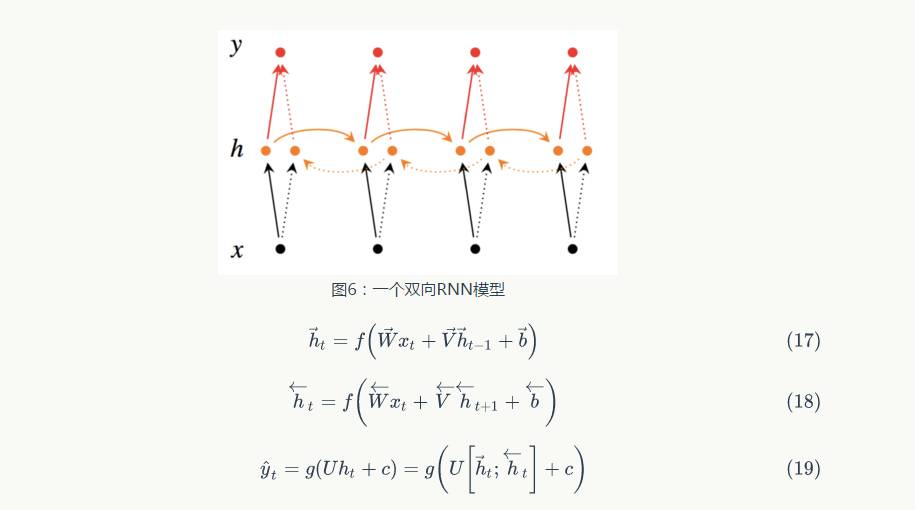
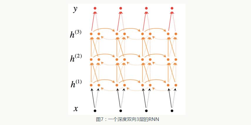
Figure 7 shows a multi-layer bidirectional RNN that propagates from lower layers to the next layer. As shown in the network structure, at time t, each intermediate neuron receives a set of parameters passed from the previous time (the same RNN layer) and two sets of parameters passed from the previous RNN layer. One set of parameters is the RNN input from left to right, and the other set is the RNN input from right to left.
To construct an L-layer RNN, the above relationships will be modified according to formulas 20 and 21, where the input of each intermediate neuron (the i-th layer) is the output of the same t-th moment of the RNN network in the (i-1)-th layer. The output at each moment is the result of the propagated input parameters through all hidden layers (as shown in formula 22).
2.4 Application: RNN Translation Model
Traditional translation models are quite complex, consisting of many machine learning algorithms applied at different stages of the language translation process. In this chapter, we discuss the potential application of RNNs to replace traditional machine translation modules. Consider the RNN example shown in Figure 8. Here, the German phrase “Echt dicke Kiste” is translated into English as “Awesome sauce.” The first three moments of the hidden layer network encode the German into some language features ( ). The final two moments decode it into English as output. Formulas 23, 24, and 25 show the encoding phase and decoding phase.
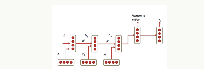
Figure 8: An RNN translation model. The first three RNN hidden layers belong to the resource language model encoder, and the last two belong to the target language model decoder.

The RNN model using the cross-entropy function (as shown in formula 26) has a high accuracy in translation results. In practice, using some extended methods on the model can improve the accuracy of translations.

Extension 1: The encoder and decoder train different RNN weights. This will decouple the two units while both RNN modules will have higher accuracy. This means that the functions in formulas 23 and 24 have different matrices.
Extension 2: Use three different inputs to calculate each hidden layer state during the encoding process:
• Previous hidden layer state (standard)
• Previous encoder’s hidden layer (in Figure 9,  )
)
• Previously predicted output word, 
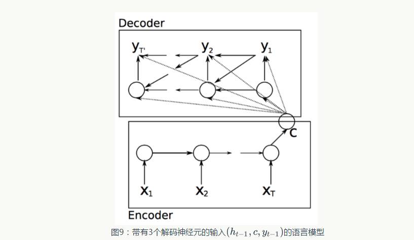
Combining the above three inputs transforms the decoding phase’s f function in formula 24 into one in formula 27. Figure 9 illustrates this model.
Extension 3: As previously discussed in this chapter, training deep recurrent neural networks using multiple RNN layers. Because deeper layers can learn more, they often improve prediction accuracy, though this also means larger corpora are required to train the model.
Extension 4: As mentioned earlier in this chapter, training bidirectional encoders to improve accuracy.
Extension 5: Given a sequence of words ABC in German, translated to XY in English, we use CBA->XY instead of ABC->XY to train the RNN. The purpose of this approach is that A is most likely to be translated to X, and considering the previously mentioned gradient vanishing problem, reversing the input word order can reduce the error rate in the output phase.
◆ ◆ ◆
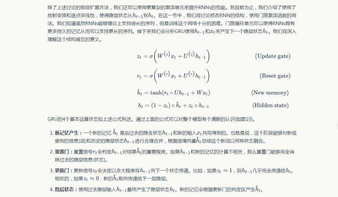
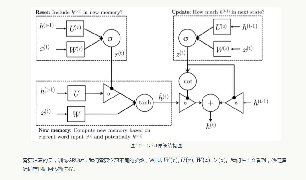
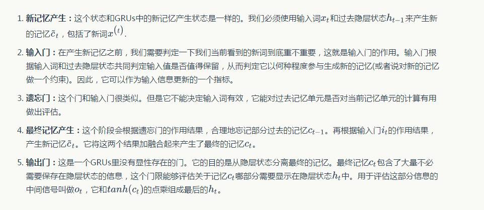
3. Gated Recurrent Unit (GRU)
◆ ◆ ◆
3. Long Short-Term Memory (LSTM)
Regarding Reproduction

If you need to reproduce this article, please prominently indicate the author and source at the beginning (reprint from: Big Data Digest | bigdatadigest), and place a prominent QR code from Big Data Digest at the end of the article. For articles without an original identification, please edit according to the reproduction requirements and can be directly reproduced; after reproduction, please send us the reproduction link; for articles with original identification, please send 【Article Name - Name and ID of the Authorized Public Account】 to apply for whitelist authorization. Unauthorized reproduction and adaptation will be pursued legally. Contact email: [email protected].
◆ ◆ ◆
Big Data Article Stanford Deep Learning Course Team
Big Data Digest backend replies “Volunteer“, to learn how to join us
Column Editor


Translator Team