Prediction Model for Greenhouse Tomato Growth Based on KNN-SVM Algorithm

China’s greenhouse vegetable industry is developing rapidly, and tomatoes are one of the typical crops in greenhouses. Tomatoes are important economic vegetable crops, with China’s planting yield and scale ranking first in the world, playing an increasingly important role in farmers’ income. Currently, the degree of data visualization in greenhouse tomato planting management is low, and environmental parameters required for growth are difficult to control accurately, severely affecting the further development of the greenhouse crop industry. To predict the growth model of tomatoes, the author collected environmental information during the seedling, flowering, and fruiting periods of greenhouse tomatoes from the experimental field of Jilin Agricultural Science and Technology College, and combined information technology with manual methods to collect full-cycle growth information of greenhouse tomatoes, studying growth models for each period of greenhouse tomatoes to provide a reference for standardized planting.

Smart Greenhouse

The smart greenhouse provides raw data for the construction of the greenhouse tomato planting model and also provides an experimental platform to verify the effectiveness of the model. The smart greenhouse mainly includes soil temperature and humidity sensors, air temperature and humidity sensors, carbon dioxide sensors, and light sensors. The smart greenhouse has network communication capabilities and can monitor environmental data in real-time, allowing for control of environmental parameters such as temperature and humidity inside the greenhouse. Tomatoes are planted in the greenhouse, and the growth status of tomatoes is recorded regularly.

Acquisition and Processing of Tomato Growth Data

2.1 Acquisition of Tomato Growth Data

The study used greenhouse data from 2020 to 2021. The tomato data is based on fruit’s transverse diameter, longitudinal diameter, moisture content, and fresh weight. Figure 1 shows the environmental data collection in the greenhouse. The dependent variable is the temperature and humidity inside the greenhouse, and the independent variables are the fruit growth data. This project uses the correlation between soil temperature and humidity in the greenhouse and tomato fruit to calibrate the quality of greenhouse tomato growth, aiming to obtain a more efficient growth model.

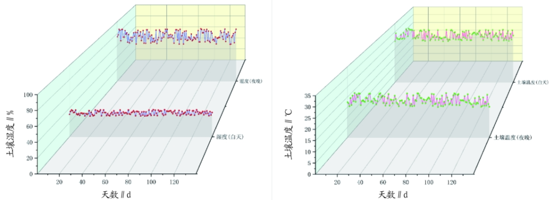
Figure 1 Greenhouse Data

2.2 Data Preprocessing

First, from the collected actual environmental data as shown in Figure 2, the KNN algorithm is used to process outliers, exclude erroneous data, and fill in all missing values as shown in Figure 3, with the fruit data being actual measurement data as shown in Figure 4.

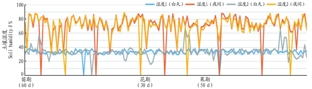
Figure 2 Soil Humidity Sensor Data

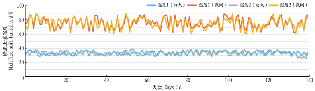
Figure 3 Corrected Soil Humidity Sensor Data

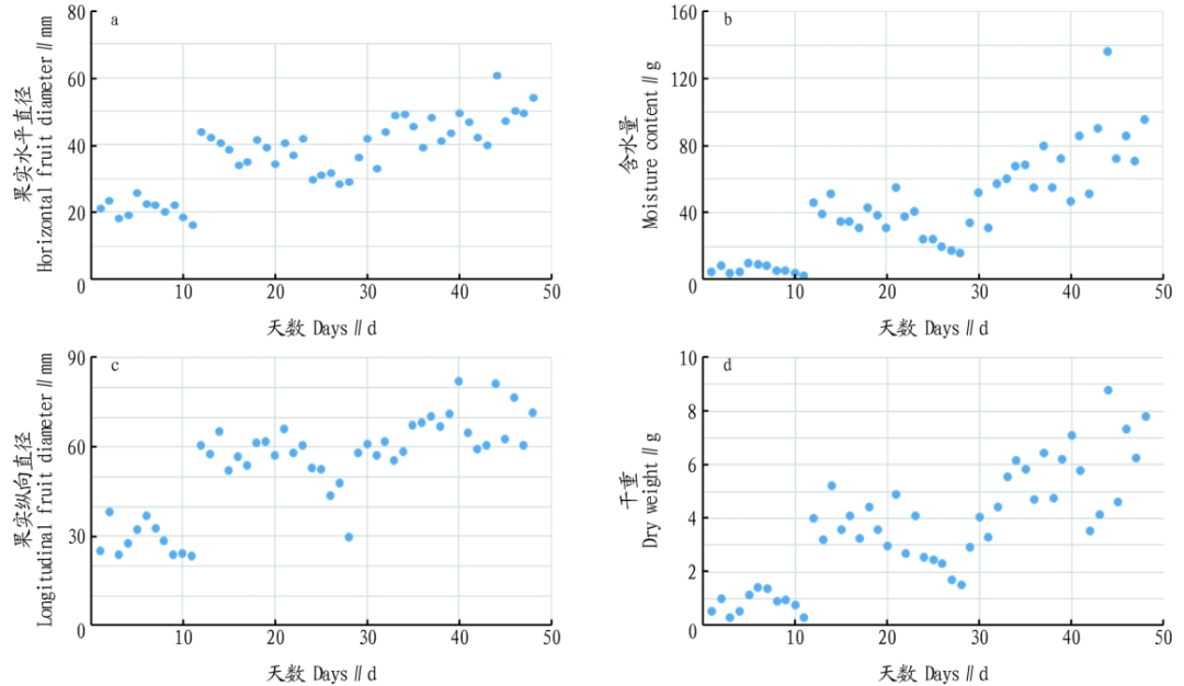
Figure 4 Tomato Fruit Data

Removing these outliers will improve the accuracy of predictions. In the entire growth process of greenhouse tomatoes, environmental data and growth data that exceed 3 standard deviations from the mean will be omitted.

Construction of the Tomato Growth Model

3.1 Correlation Analysis of Tomato Growth Model

The Pearson correlation coefficient is used to explain the linear correlation degree between two random variables, with values ranging from -1 to 1. Let there be two variables X and Y, then the relationship of the Pearson correlation coefficient between X and Y is as follows:

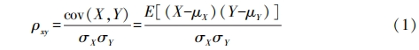
In the above formula, cov(X,Y) is the covariance of X and Y, σ_X is the standard deviation of X, and σ_Y is the standard deviation of Y. The test to determine whether the observed data follows a normal distribution is called normality testing, with the common normality test method being the Shapiro-Wilk test. This test has two basic hypotheses: H0 states that the sample comes from a population that follows a normal distribution; H1 states that the sample comes from a population that does not follow a normal distribution. Table 1 shows the results of the Shapiro-Wilk test on the tomato growth data. From Table 1, it can be seen that the w values of all variables approach 1, and the P value is greater than 0.05, conforming to H0, indicating that the overall sample follows a normal distribution, thus meeting the prerequisites for using the Pearson correlation coefficient.

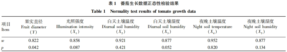
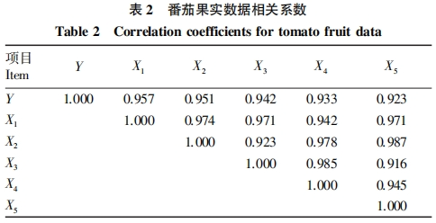
Table 2 shows the correlation coefficients between each variable of the tomato growth data. It can be seen from Table 2 that the correlation coefficients between the diameter of greenhouse tomato fruits and various environmental factors are 0.957, 0.951, 0.942, 0.933, and 0.923, indicating a strong correlation between the growth of greenhouse tomatoes and each environmental factor.

The input parameters include fruit’s transverse diameter, longitudinal diameter, humidity, and temperature. The correlation coefficients between the growth environment and crop growth are shown in Figure 5.

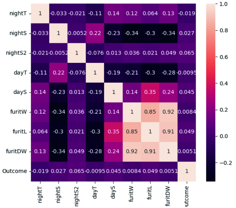
Figure 5 Correlation Heatmap

In Figure 5, nightT is the night soil temperature, nightS is the night soil humidity, dayT is the daytime soil temperature, dayS is the daytime soil humidity, fruitW is the fruit weight, fruitL is the fruit diameter, fruitDW is the fruit dry weight, and Outcome is the output of healthy growth. From Figure 5, it can be seen that the tomato label Outcome (healthy growth) has a large positive correlation coefficient with daytime soil humidity dayS, indicating that within a certain range, tomato growth is positively correlated with humidity. Similarly, the correlation between soil humidity dayS and fruit diameter fruitL is also strong.

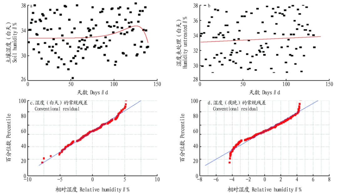
Figure 6 Linear Model of Environmental Parameter Variables

3.2 Significance of Linear Discriminant Analysis

Linear Discriminant Analysis (LDA) is a supervised linear dimensionality reduction algorithm. LDA aims to make the data points after dimensionality reduction as distinguishable as possible. Its principle is to project the samples onto a line in such a way that the projections of the same class are as close as possible, while the projections of different classes are as far apart as possible; when classifying new samples, project them onto this line and determine the class of the new sample based on the position of the projection point. The LDA technique is applied to analyze the sample data of greenhouse tomatoes, with the dataset including 250 data points divided into 5 classes, each class containing 50 data points, and each data point containing 5 attributes. The goal of the analysis is to classify by mapping the input matrix into a lower-dimensional space using the LDA algorithm.

3.3 Significance of Support Vector Machines

Support Vector Machine (SVM) is a commonly used machine learning algorithm, whose basic idea is to construct an optimal hyperplane in a high-dimensional space to achieve data classification. More specifically, SVM has two implementation methods: linear SVM and nonlinear SVM. The linear SVM method solves the optimal hyperplane by maximizing the distance from the data points to the hyperplane, while the nonlinear SVM method maps the data into high-dimensional space using kernel functions in order to find the optimal hyperplane in high-dimensional space.

As shown in Figure 7, data preprocessing is first performed, calculating the sample mean vector for each class and the overall sample mean vector, then calculating the within-class scatter matrix and the between-class scatter matrix, and finally training the model for evaluation. Figure 7b introduces the structure of the LR algorithm, which first undergoes data preprocessing, such as feature scaling and handling missing values, then trains the model using maximum likelihood estimation or gradient descent to estimate model parameters, and finally evaluates the model using test set data. Figure 7c introduces the structure of the improved SVM algorithm, which evaluates the SVM model through various combinations of hyperparameter tuning and uses cross-validation for verification. This study meticulously adjusted two hyperparameters of the SVM model until achieving the best accuracy. In the SVM model, the kernel function cache was first implemented to cache the most computationally intensive kernel function calculations, improving efficiency by 20 times. Secondly, the optimization of error value solving was defined.

To find a partial derivative of g(x) with respect to a, if a_i and a_j change by a step size delta, then all samples corresponding to g(x) are updated by adding delta multiplied by the partial derivatives with respect to a_i and a_j. After successfully updating a pair of a_i and a_j, all samples corresponding to g(x) are updated in the cache, thus avoiding a large amount of redundant computation through each iteration update of g(x).

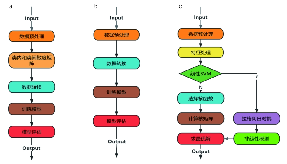
Figure 7 Algorithm Structure

Results and Analysis

This study explores the role of greenhouse environments in crop growth, using the SVM algorithm to predict the growth model of greenhouse tomatoes. It analyzes machine learning methods that can help improve environmental control of temperature or humidity during tomato growth in greenhouses. During the day, as the temperature rises, the relative humidity in the soil decreases; at night, as the temperature decreases, the relative humidity in the soil increases. This study establishes a reliable greenhouse tomato growth simulation model based on real-time weights. The values generated by the SVM model can accurately simulate the total weight of tomato plants. The model has few parameters, good fitting effect, and strong predictability, providing effective means for predicting the real-time weight of tomatoes and helping researchers understand the daily growth rate of tomatoes, directly determining the growth rate of tomatoes. Without disrupting the normal growth of tomato plants, it allows timely understanding of the growth status of tomato fruits, predicting fruit weight, and simulating the accumulation of dry matter, providing a basis for reasonable management. The model can be used to visually describe the growth of tomatoes; to predict the growth of other different crops, different parameters should be used.

The machine learning model provides a method to calculate the impact of predictors on the overall model. After arranging each predicted value, the process is repeated, and the accuracy differences of all models are averaged and normalized through standard error. Hyperparameter tuning is searched to select an approximately optimal configuration for each classifier. Based on empirical research, the tuning parameters for the SVM model produced the best accuracy model, as shown in Figure 8. Models with large-dimensional hyperparameter search spaces will train the SVM model.

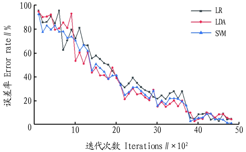
Figure 8 Cross-Validation of Classification Accuracy

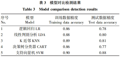
From Table 3, it can be seen that the SVM classifier outperforms other machine learning classifiers. The accuracy of SVM is the highest at 0.90. The accuracies of LR and LDA are 0.86 and 0.88, respectively. In this test, SVM is a kernel function-based machine learning model that can serve as an effective method for predicting the growth of greenhouse tomatoes. Among the correlations of different environmental parameters, such as air temperature and humidity, soil temperature and humidity, and light intensity, the accuracy of SVM model training is 0.90, with an accuracy of 0.88 in the test data, both showing the best estimation accuracy. The testing accuracy values for tomato growth of SVM, LR, and LDA models also differ. The SVM model (testing accuracy 0.88) outperforms the LR model (testing accuracy 0.78) and is slightly better than the LDA model (testing accuracy 0.80). Due to the advantages of the SVM model in simulating the dynamic nonlinear interactions between greenhouse tomato growth and environmental variables, it is more suitable for regular estimation of tomato growth.

Conclusion

The proposed prediction model outperforms other prediction models in terms of accuracy, with a prediction accuracy of 0.90. The KNN-SVM model is key to achieving accurate predictions, indicating that the performance of the model can be improved by designing the model architecture.