Full Article Link: https://tecdat.cn/?p=33917

KNN is a non-parametric learning algorithm, which means it makes no assumptions about the underlying data. This is a very useful feature because most client data does not really follow any theoretical assumptions, such as linear separability, uniform distribution, etc. (Click the “Read the Original” link at the end of the article to get the complete code data).

Related Videos

When to Use KNN?

Suppose you want to rent an apartment and have recently discovered that your friend’s neighbor may be renting her apartment in two weeks. Since the apartment has not yet appeared on the rental website, how would you try to estimate its rent?

Assuming your friend pays $1,200 in rent. Your rent value might be about that number, but the apartments are not exactly the same (direction, area, furniture quality, etc.), so it would be good to have data on more other apartments.

By asking other neighbors and checking the apartments listed on rental websites in the same building, the rents of the three closest neighbors’ apartments are $1,200, $1,210, $1,210, and $1,215. These apartments are in the same block and floor as your friend’s apartment.

The rents of other apartments on the same floor but in different blocks are $1,400, $1,430, $1,500, and $1,470. They seem more expensive because they receive more sunlight in the evening.

Considering the proximity of the apartments, you estimate that your rent should be around $1,210. This is the general idea of the K-Nearest Neighbors (KNN) algorithm!

Housing Dataset

We will use the housing dataset to illustrate how the KNN algorithm works. This dataset originates from the 1990 census. A row in the dataset represents a census of a block.

Block groups are the smallest geographic units for which the Census Bureau publishes sample data. In addition to block groups, there is a variable for households, which are groups of people living in the same house.

The dataset contains nine attributes:

• MedInc – Median income for each block.

• HouseAge – Median age of houses in each block.

• AveRooms – Average number of rooms per household.

• AveBedrms – Average number of bedrooms per household.

• Population – Population of the block.

• AveOccup – Average number of members living in each household.

• Latitude – Latitude of the block.

• Longitude – Longitude of the block.

• MedHouseVal – Median house value (in thousands).

Let’s import Pandas and take a look at the first few rows of data:

df.head()

Executing this code will display the first five rows of our dataset:

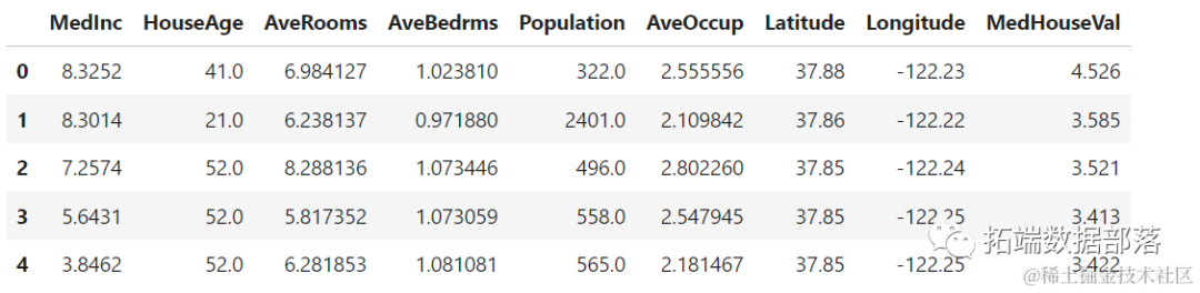
We will use MedInc, HouseAge, AveRooms, AveBedrms, Population, AveOccup, Latitude, Longitude to predict MedHouseVal.

Now, let’s directly implement the KNN regression algorithm.

Using Scikit-Learn for K-Nearest Neighbors Regression

So far, we have understood the dataset, and we can now proceed with the other steps of the KNN algorithm.

Preprocess Data for KNN Regression

y = df['MedHouseVal']

For feature standardization, we will use the StandardScaler class from Scikit-Learn later.

Split Data into Training and Test Sets

To standardize the data without leakage, while evaluating our results and avoiding overfitting, we will split the dataset into training and testing sets.

To make this process reproducible (to sample the same data points every time), we will set the random_state parameter to a specific SEED:

X_train, X_test, y_train, y_test = train_test_split(X, y, test_size=0.25, random_state=SEED)

This code will use 75% of the data for training and 25% for testing. By changing the test_size to 0.3, for example, you can use 70% of the data for training and 30% for testing.

Now we can fit the data standardization on the X_train dataset and standardize both X_train and X_test.

Feature Standardization for KNN Regression

By importing StandardScaler, instantiating it, fitting it to our training data, and transforming the training and testing datasets, we can perform feature standardization:

# Fit only on X_train
scaler.fit(X_train)

# Standardize X_train and X_test
X_test = scaler.transform(X_test)

Now our data has been standardized.

Training and Predicting with KNN Regression

Fit to our training data:

regressor.fit(X_train, y_train)

The final step is to predict our test data. To do this, execute the following script:

predict(X_test)

Now we can evaluate our model’s generalization ability on new data with labels (true values) – that is, the test set!

Evaluating KNN Regression Algorithm

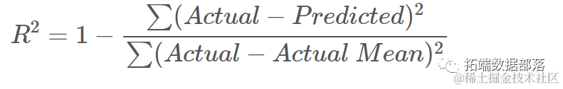
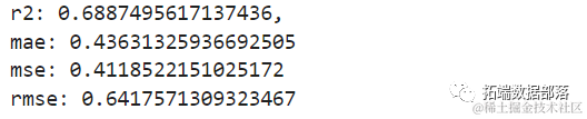
The most commonly used regression metrics for evaluating the algorithm are Mean Absolute Error (MAE), Mean Squared Error (MSE), Root Mean Squared Error (RMSE), and R-squared (R2).

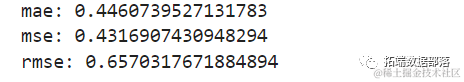
You can calculate these metrics using the mean_absolute_error() and mean_squared_error() methods from sklearn.metrics, as shown in the code snippet below:

print(f'mse: {mse}')
print(f'rmse: {rmse}')

The output of the above script is as follows:

You can directly calculate R2 using the score() method:

regrscore(X_test, y_test)

The output is as follows:

The mean is 2.06 with a standard deviation of 1.15, so our score is about 0.44, which is neither very good nor too bad.

For R2, the closer the score is to 1 (or 100), the better. R2 indicates how much of the data variance the KNN can understand (explain).

The score is 0.67, and we can see that the model explains 67% of the data variance. This is already above 50%, which is good, but not very good. Can we have other methods to improve the prediction effect?

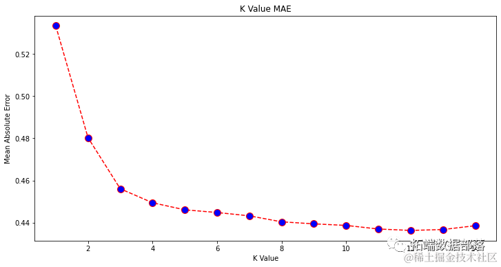
To determine the ideal K value, we can analyze the algorithm’s error and select the K that minimizes the loss.

Finding the Best K Value

To do this, we will create a for loop and run models with neighbors ranging from 1 to X. In each iteration, we will calculate the MAE and plot the K values along with the MAE results:

error = []

# Calculate MAE error for different k
for i in range(1, 40):
 ......
    error.append(mae)

Now, let’s plot error:

import matplotlib.pyplot as plt

plt.figure(figsize=(12, 6))
......
plt.ylabel('Mean Absolute Error')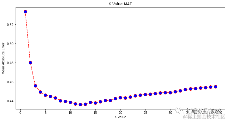

Click the title to check past content

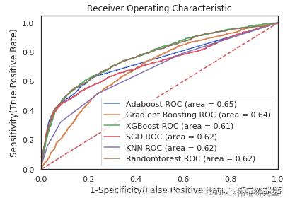
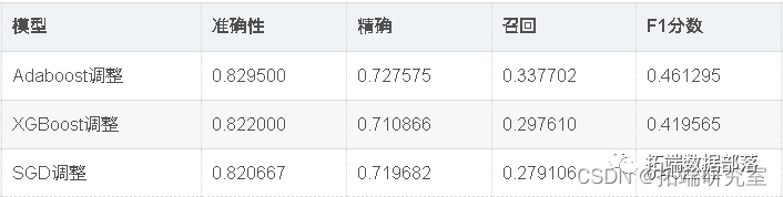
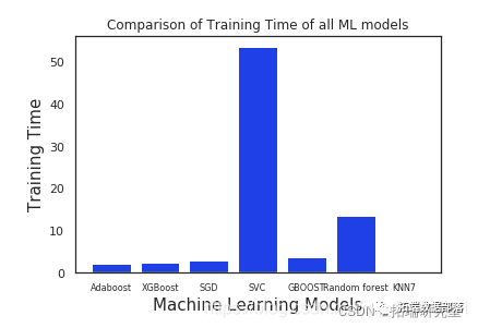
Python Credit Risk Control Model: Adaboost, XGBoost, SGD, SVC, Random Forest, KNN Predicting Credit Default Payment

Swipe left and right to see more

01

02

03

04

Looking at the chart, when the K value is 12, it seems to have the smallest mean absolute error (MAE). Let’s take a closer look at the chart by plotting less data to confirm:

plt.figure(figsize=(12, 6))
......

You can also use the built-in min() function (for lists) to get the minimum error and its index, or convert the list to a NumPy array and use the argmin() function (to find the index of the element with the minimum value):

import numpy as np
......
print(np.array(error).argmin()) # 11

We start counting neighbors from 1, while the array starts from 0, so the 11th index is 12 neighbors!

This means we need 12 neighbors to predict a point with the minimum MAE error. We can again use 12 neighbors to execute the model and metrics to compare the results:

knn_reg12 = KNei......
print(f'r2: {r2}, 
mae: {mae12} 
mse: {mse12} 
rmse: {rmse12}')

The following code outputs:

We have seen how to use KNN for regression, but what if we want to classify a point instead of predicting its value? Now we can look at how to use KNN for classification.

Using Scikit-Learn for K-Nearest Neighbors Classification

In this task, we are no longer predicting continuous values but want to predict the categories to which these block groups belong. To do this, we can group the median house values of the areas into different house value ranges or “bins”.

Preprocess Data for Classification

Let’s create bins for the data that will convert continuous values into categories:

# Create 4 categories and assign them to MedHouseValCat column
df["MedHouseValCat"] = pd.cut(df["MedHouseVal"], bins=4, labels=[1, 2, 3, 4])

Then, we can split the dataset into attributes and labels:

y = df['MedHouseValCat']
X = df.drop(['MedHouseVal', 'MedHouseValCat'], axis=1)

Since we created bins using the MedHouseVal column, we need to remove the MedHouseVal column and the MedHouseValCat column from X.

Split Dataset into Training and Test Sets

Similar to regression, we will also split the dataset into training and test sets. Since we have different data, we need to repeat this process:

from sklearn.model_selection import train_test_split
X_train, X_test, y_train, y_test = train_test_split(X, y, test_size=0.25, random_state=SEED)

We will again use the standard Scikit-Learn values, i.e., 75% training data and 25% test data. This means that the number of training and test records will be the same as before for regression.

Feature Standardization for Classification

Since we are dealing with the same unprocessed dataset and its different measurement units, we will again perform feature standardization in the same way as before for regression data:

from sklearn.preprocessing import StandardScaler
scaler = StandardScaler()
scaler.fit(X_train)
X_train = scaler.transform(X_train)
X_test = scaler.transform(X_test)

Training and Predicting for Classification

After binning, splitting, and standardizing the data, we can finally fit a classifier on it. For prediction, we will again use 5 neighbors as a baseline. You can also instantiate the KNeighborsClassifier class without any parameters, and it will automatically use 5 neighbors. This time, we will import the KNeighborsClassifier class instead of the KNeighborsRegressor:

from sklearn.neighbors import KNeighborsClassifier
classifier = KNeighborsClassifier()
classifier.fit(X_train, y_train)

After fitting, we can predict the categories of the test data:

Evaluating KNN for Classification

To evaluate the KNN classifier, we can use the score method, but it performs different metrics since we are scoring a classifier rather than a regressor.

Let’s score our classifier:

acc = classifier.score(X_test, y_test)
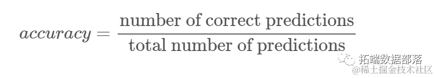
print(acc)  # 0.6191860465116279

By observing the score results, we can infer that our classifier predicts about 62% of the categories correctly. This already helps in analysis, although just knowing what the classifier predicts correctly does not easily improve it.

We can use other metrics to delve deeper into the results to determine. Here, we will use different steps from regression:

1. Confusion Matrix: Understand how well we predict correctly or incorrectly for each category. The values that are correctly predicted are called true positives, while those predicted as positive but are not positive are called false positives. Similarly, true negatives and false negatives are named for negative values.

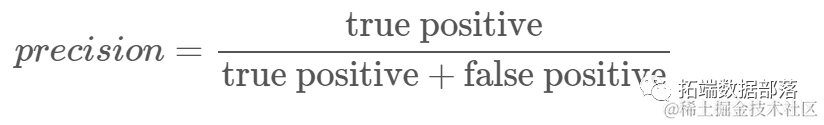
1. Precision: Understand which correct predicted values the classifier thinks are correct. Precision divides the true positive values by any values predicted as positive;

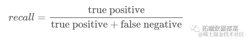
2. Recall: Understand how many true positives the classifier identifies. Recall is calculated by dividing true positives by any values that should be predicted as positive.

1. F1 Score: This is the balance or harmonic mean of precision and recall. The minimum value is 0, and the maximum value is 1. When the f1-score equals 1, it means all categories are predicted correctly – this is a score that is very hard to achieve with real data (there will almost always be exceptions).

To obtain metrics, execute the following code snippet:

## Import Seaborn for heatmap visualization
import seaborn as sns

# Add category names for better interpretation
classes_names = ['class 1', 'class 2', 'class 3', 'class 4']

# Use Seaborn's heatmap to better visualize the confusion matrix
sns.heatmap(confusion_matrix(y_test, y_pred), annot=True, fmt='d');

print(classification_report(y_test, y_pred)

The output of the above script is as follows:

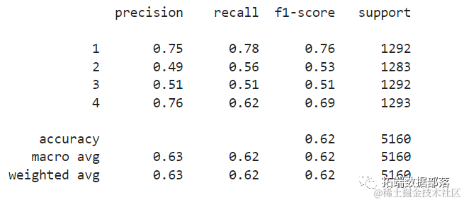
The results indicate that KNN can classify all 5,160 records in the test set with an accuracy of 62%, which is above average. The support is quite balanced (the distribution of categories in the dataset is quite uniform), so the weighted F1 and unweighted F1 will be roughly the same.

By observing the confusion matrix, we can see the following:

• Class 1 is mostly misclassified as Class 2 among 238 samples.

• Class 2 is misclassified as Class 1 among 256 samples and as Class 3 among 260 samples.

• Class 3 is mostly misclassified as Class 2 among 374 samples and as Class 4 among 193 samples.

• Class 4 is misclassified as Class 3 among 339 samples and as Class 2 among 130 samples.

Finding the Best K Value for KNN Classification

Let’s repeat the procedure we used for regression and plot the K values against the corresponding metrics of the test set. You can also choose metrics that suit your context; here we will choose f1-score.

f1s = []

# Calculate f1 score for K values between 1 and 40
for i in range(1, 40):
    ......
    # Calculate weighted average for the 4 classes using average='weighted'
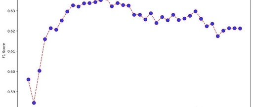
    f1s.append(f1_score(y_test, y_pred, average='weighted')

The next step is to plot the relationship between f1_score values and K values. Unlike regression, this time we are not choosing the K value that minimizes the error but rather the one that maximizes the f1-score value.

Execute the following script to create the plot:

plt.figure(figsize=(12, 6))
plt.plot(range(1, 40), f1s)
plt.ylabel('F1 Score')

The output chart is as follows:

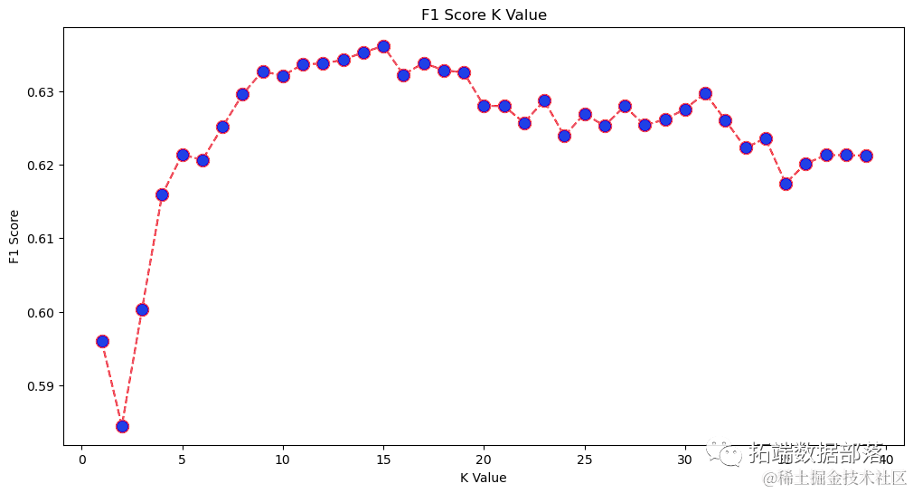
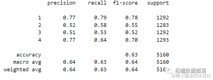
From the output, we can see that when the K value is 15, the f1-score is the highest. Let’s retrain the classifier using 15 neighbors and see the impact on the classification report results:

classifier15 = KNeighborsClassifier(n_neighbors=15)
classifier15.fit(X_train, y_train)

y_pred15 = classifier15.predict(X_test)
print(classification_report(y_test, y_pred15))

This will output the following result:

In addition to using KNN for regression and classification to determine block values and categories, we can also use KNN to detect block values that are different from the majority of the data – block values that do not follow the trend of the majority of the data. In other words, we can use KNN to detect outliers.

Implementing KNN Algorithm for Outlier Detection Using Scikit-Learn

Outlier detection uses a method that differs from the regression and classification we did previously.

After importing, we will instantiate a NearestNeighbors class with 5 neighbors – you can also instantiate it with 12 neighbors to identify outliers in the regression example or use the same operation with 15 neighbors for the classification example. Then, we will fit our training data and use the kneighbors() method to find the computed distances of each data point and neighbor indices:

nbrs.fit(X_train)
# Distances and indices of neighbors
distances, indices = nbrs.kneighbors(X_train)

Now we have 5 distances for each data point – the distances to its 5 neighbors, along with their indices. Let’s take a look at the first three results and the shape of the array for better visualization.

Execute the following code to see the shape of the first three distances:

distances[:3], distances.shape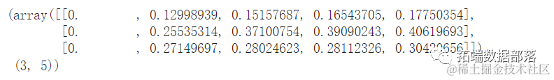

We observe that there are 3 rows, each with 5 distances. We can also look at the indices of the neighbors:

indexes[:3], indexes[:3].shape

In the above output, we can see the indices of the 5 neighbors. Now we can proceed to calculate the average of these 5 distances and plot a chart, with the X-axis counting each row and the Y-axis showing each average distance:

dist_means = distances.mean(axis=1)
plt.plot(dist_means)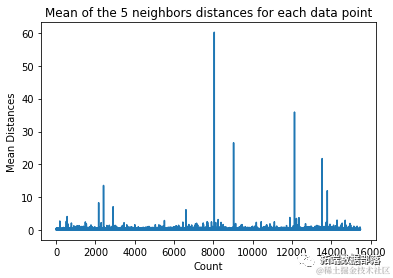

Note that there is a section in the chart where the average distances have uniform values. When the average distance is not too high and not too low, it indicates that the point is one we need to identify and remove as an outlier.

In this example, the average distance is 3. Let’s plot the chart again and use a horizontal dashed line to mark it:

plt.axhline(y=3, color='r', linestyle='--')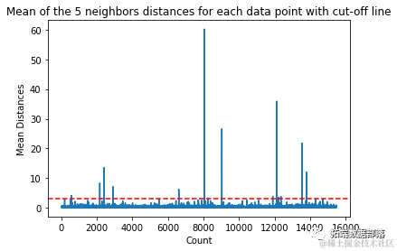

This line marks the average distance, and all values above this line are considered outliers. This means that all points with an average distance greater than 3 are outliers.

# Visually identify the cutoff value greater than 3
outlier_index = np.where(dist_means > 3)
outlier_index

The result of the above code output is:

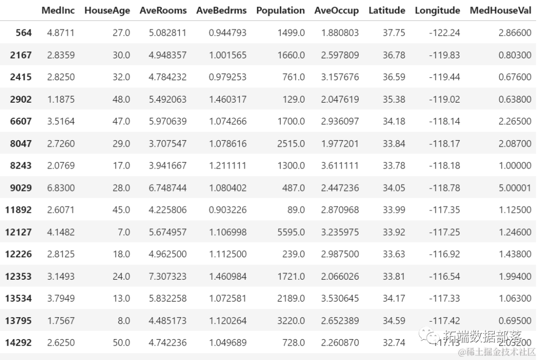
# Filter outliers
outliers = df.iloc[outlier_index]
outlier_values

Our outlier detection is complete. This is how we find each data point that does not conform to the overall data trend. We can see that there are 16 points in our training data that should be looked into, investigated, processed, or even removed from our data (if they are erroneous inputs) to improve results. These points may be due to input errors, inconsistent mean block values, or both.

Advantages and Disadvantages of KNN Algorithm

Advantages

• Simple to implement

• It is a lazy learning algorithm, so it does not require training on all data points (only uses K nearest neighbors for predictions). This makes the KNN algorithm much faster than others that require training on the entire dataset (like support vector machines and linear regression).

• Since KNN does not require training before making predictions, new data can be seamlessly added.

• Using KNN only requires two parameters: the value of K and the distance function.

Disadvantages

• The KNN algorithm performs poorly when dealing with high-dimensional data because calculating distances between points in high-dimensional space is more complex, and the distance metrics we use become less applicable.

• Finally, the KNN algorithm does not perform well when handling data with categorical features since it is difficult to calculate distances between dimensions with categorical features.

Click at the end of the article “Read the Original”

to obtain the complete code data materials.

This article is excerpted from “Predicting House Prices Using KNN for Regression, Classification, and Outlier Detection”.

Click the title to check past content

Python for Multi-Output (Multiple Dependent Variables) Regression: Ensemble Learning Gradient Boosting Decision Trees, GBR Regression Training and Prediction Visualization

Python for Store Data LSTM and XGBoost Sales Volume Time Series Modeling and Prediction Analysis

PYTHON Ensemble Machine Learning: Using ADABOOST, Decision Trees, Logistic Regression Ensemble Models for Classification and Regression and Grid Search Hyperparameter Optimization

R Language Ensemble Models: Boosting Trees, Random Forests, Constrained Least Squares Weighted Average Model Fusion Analysis of Time Series Data

Python for Store Data LSTM and XGBoost Sales Volume Time Series Modeling and Prediction Analysis

R Language Using PCA, Logistic Regression, Decision Trees, Random Forests to Analyze Heart Disease Data and High-Dimensional Visualization

R Language Tree-Based Methods: Decision Trees, Random Forests, Bagging, Boosted Trees

R Language Using Logistic Regression, Decision Trees, and Random Forests for Classification Prediction on Credit Datasets

SPSS Modeler Using Decision Trees and Neural Networks to Predict ST Stocks

R Language Using Linear Models, Regression Decision Trees to Automatically Combine Feature Factor Levels

R Language Implementing Custom Gini Coefficient CART Regression Decision Trees

R Language Using Poisson Regression, GAM Spline Curve Models to Predict the Number of Cyclists

R Language Quantile Regression, GAM Spline Curves, Exponential Smoothing, and SARIMA for Power Load Time Series Prediction

R Language Spline Curves, Decision Trees, Adaboost, Gradient Boosting (GBM) Algorithms for Regression, Classification, and Dynamic Visualization

How to Build Ensemble Models in Machine Learning with R Language?

R Language ARMA-EGARCH Model, Ensemble Prediction Algorithms for Predicting Actual Volatility of SPX

Calculating Neural Network Ensemble Models in Python Deep Learning Keras

R Language ARIMA Ensemble Model for Time Series Analysis

R Language Using Bagging Classification of Logistic Regression, Decision Trees, Forests to Analyze Heart Disease Patients

R Language Tree-Based Methods: Decision Trees, Random Forests, Bagging, Boosted Trees

R Language Bootstrap-Based Linear Regression Prediction Confidence Interval Estimation Methods

R Language Using Bootstrap and Incremental Methods to Calculate Generalized Linear Model (GLM) Prediction Confidence Intervals

R Language Spline Curves, Decision Trees, Adaboost, Gradient Boosting (GBM) Algorithms for Regression, Classification, and Dynamic Visualization

Python for Store Data LSTM and XGBoost Sales Volume Time Series Modeling and Prediction Analysis

R Language Random Forest RandomForest, Logistic Regression Logistic Predicting Heart Disease Data and Visualization Analysis

R Language Using PCA, Logistic Regression, Decision Trees, Random Forests to Analyze Heart Disease Data and High-Dimensional Visualization

Matlab Building SVM, KNN, and Naive Bayes Model Classification Drawing ROC Curves

Matlab Using Quantile Random Forest (QRF) Regression Tree to Detect Outliers