
Hello everyone, I am Xiao Wu Ge. It has been a while since my last update. Recently, I have been looking at various topics, and I don’t know where to start. I have been quite busy with work, but I managed to find some time this weekend to write an article.
Most of the articles online about Graph Neural Networks are experiments on datasets like Cora and Citeseer, which are ideal datasets that have already been processed. They look clear, but when applied to real business scenarios, beginners find it difficult to start. This is because the hardest part of Graph Neural Networks is processing your own data into a standard format that the algorithm can use. This step can be even more challenging than training the Graph Neural Network. Today, I will create a small dataset and write a template for GCN for everyone to reference. The data format for this session is as follows:
First, we need to read the dataset. If you need a sample of the csv data, please reply with 【Graph Data】 in the backend:
# Follow Xiao Wu Ge for risk control discussions, reply with 【Graph Data】 in the backend
import pandas as pd
# Training set operation detail form
data = pd.read_csv('Graph Neural Network Sample.csv')
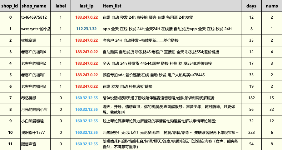
data.head(12)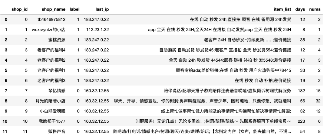
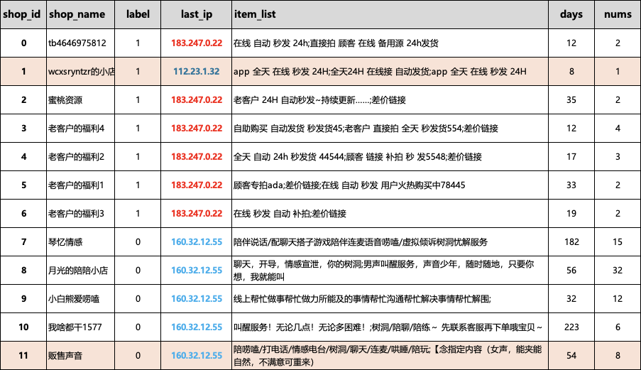
The dataset is organized by myself, and it contains samples from 12 merchants. 1 represents black samples (most likely to be fraudulent), and 0 represents white samples. The IP is the medium here, and we use IP to construct a homogeneous graph, then use product title, registration duration, and product quantity as features for training, validation, and prediction.
Data Construction
By matching based on last_ip, we can perform a simple conversion to a homogeneous graph. Of course, in actual business scenarios, there may be more complex and specialized construction requirements. You can refer to my course, where I discuss six different construction methods.Everything is a network
# Follow Xiao Wu Ge for risk control discussions, reply with 【Graph Data】 in the backend
da = data[['shop_name','last_ip']]
# Match based on keywords
df_join = da.merge(da,on='last_ip')
#df_join = df_join[df_join['shop_name_x']!=df_join['shop_name_y']]
df_join = df_join[['shop_name_x','shop_name_y']]
df_join.head()
shop_name_x shop_name_y
0 tb4646975812 tb46469758121
1 tb4646975812 蜜桃资源
2 tb4646975812 老客户的福利
3 tb4646975812 老客户的福利
4 tb4646975812 老客户的福利
5 tb4646975812 老客户的福利
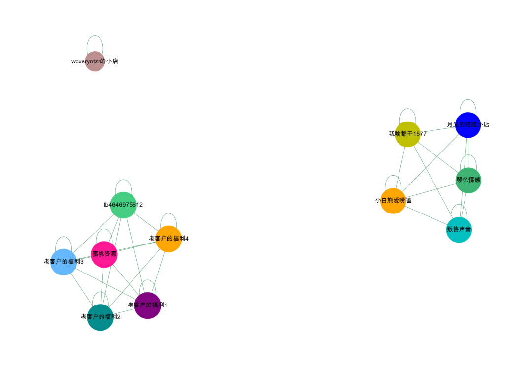
1A simple visualization shows that there are roughly two groups and one isolated point. The Graph Neural Network can predict isolated nodes well by adding self-loops, and we will look at the results shortly.
Node Encoding
What we have obtained above is the relationship with Chinese names. Our DGL framework requires the input nodes to be in numeric format, so we need to encode the nodes numerically. Of course, we can also write a decoding function to restore the numbers. The scr and dst sequences are the starting and destination nodes we will use in the graph construction. df_join is used to restore the encoded numbers, making it clearer for everyone. For example, the merchant name:tb4646975812 has an encoded node ID of 0.
# Encoding method
def encode_map(idx):    p_map = {}
for index, ele in zip(range(len(idx)),idx):        p_map[ele] = index
return p_map

# Decoding method
def decode_map(encode_map):    de_map={}
for k,v in encode_map.items():         de_map[v]=k
return de_map

# Encode nodes
dic = encode_map(data['shop_name'])
print(dic)
#{'tb4646975812': 0, 'wcxsryntzr的小店': 1, '蜜桃资源': 2, '老客户的福利4': 3, '老客户的福利2': 4, '老客户的福利1': 5, '老客户的福利3': 6, '琴忆情感': 7, '月光的陪陪小店': 8, '小白熊爱唠嗑': 9, '我啥都干1577': 10, '贩售声音': 11}
df_join['scr_encode'] = df_join['shop_name_x'].apply(lambda x:dic[x])
df_join['dst_encode'] = df_join['shop_name_y'].apply(lambda x:dic[x])
scr = df_join['scr_encode'].to_numpy()
dst = df_join['dst_encode'].to_numpy()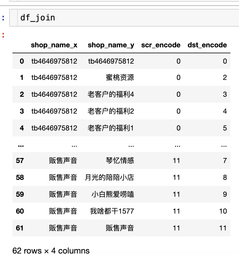
Constructing DGL Graph
Based on the encoded nodes, we construct a DGL graph.
import dgl
# DGL graph construction
g  = dgl.graph((scr,dst))
# Add self-loops, otherwise some nodes cannot be predicted
g = dgl.add_self_loop(g)
print(g)
# Remove duplicates using the to_bidirected function; can also use nx to remove
g  = dgl.to_bidirected(g)
print(g)
Feature Engineering
The basic graph is built, and we need to focus on processing feature engineering. The features include text and numeric data; we will first process the text.
# Load Jieba for word segmentation
import jieba
# Perform word segmentation
data['text'] = data['item_list'].apply(lambda x: ' '.join(jieba.cut(x)))
data.head()
# CountVectorizer can calculate the occurrence of each word
from sklearn.feature_extraction.text import TfidfVectorizer,CountVectorizer
# Initialize vectorizer
vectorizer = CountVectorizer(max_features=25,token_pattern=r"(?u)\b\w+\b",min_df = 1, analyzer='word')
# Train the vectorizer
vectorizer.fit(data['text'])
# Convert words into CountVectorizer vectors
feat_item = vectorizer.transform(data['text'])
len(vectorizer_word.vocabulary_)
feat_item = pd.DataFrame(feat_item.toarray())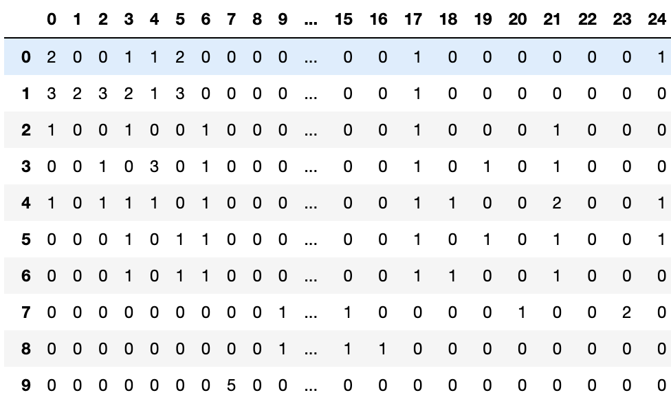
It may not be very clear, so let’s reverse the words back to see.
# Reverse the dictionary
onehotdic = {}
for k,v in vectorizer_word.vocabulary_.items():    onehotdic[v] = k
    feat_item.columns = [onehotdic[i] for i in list(feat_item.columns)]
feats = pd.concat([feat_item,data[['days','nums']]],axis=1)
feats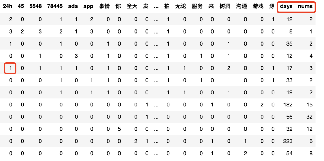
Each word represents the count of that word in each sample, and when combined with our numeric features, we limit the words to the top 25, resulting in a total of 27 dimensions. Features for Graph Neural Networks need to be normalized.
import pandas as pd
from sklearn.preprocessing import MinMaxScaler
transfer = MinMaxScaler(feature_range=(0, 1))   # Instantiate a transformer class
features = transfer.fit_transform(feats)   # Call fit_transform
features
Then convert it to tensor format, so our graph, features, and labels are ready. Next, we will start dividing the training set, validation set, and test set.
import pandas as pd
from sklearn.preprocessing import MinMaxScaler
transfer = MinMaxScaler(feature_range=(0, 1))   # Instantiate a transformer class
features = transfer.fit_transform(feats)   # Call fit_transform
features
Dataset Division
The mask operation is equivalent to the training set, validation set, and test set division in conventional machine learning.
# Mask operation, equivalent to the training set, validation set, and test set division in conventional machine learning
def sample_mask(idx, l):    """Create mask."""
    mask = np.zeros(l)
    mask[idx] = 1
    return np.array(mask,dtype=np.bool_)
#[ Black 0, 1, 2, 3, 4, 5, 6,  White 7, 8, 9, 10, 11] 0-6 are black samples, 7-11 are white samples, 1 is an isolated sample
# 0 2
idx_train = [0,2,3,4,7,8,9]
idx_val   = [5,6,10]
idx_test  = [1, 11]
train_mask = sample_mask(idx_train, 12)
val_mask   = sample_mask(idx_val, 12)
test_mask  = sample_mask(idx_test, 12)
masks    = train_mask,val_mask,test_mask
Next is the model construction; there is already a lot of information available online, so I won’t elaborate further, as you can find information anywhere.
import os
import numpy as np
import pandas as pd
import torch
import scipy.sparse as sp
import dgl
import argparse
import torch
import torch.nn as nn
import torch.nn.functional as F
import dgl.nn as dglnn
from dgl import AddSelfLoop
from dgl.data import CoraGraphDataset
torch.set_default_tensor_type(torch.DoubleTensor)

device   = torch.device('cuda' if torch.cuda.is_available() else 'cpu')
in_size  = features.shape[1]
out_size = 2


class GCN(nn.Module):    def __init__(self, in_size, hid_size, out_size):        super().__init__()        self.layers = nn.ModuleList()        # two-layer GCN        self.layers.append(dglnn.GraphConv(in_size, hid_size, activation=F.relu))        self.layers.append(dglnn.GraphConv(hid_size, out_size))        self.dropout = nn.Dropout(0.3)
    def forward(self, g, features):        h = features        for i, layer in enumerate(self.layers):            if i != 0:                h = self.dropout(h)            h = layer(g, h)        #h = F.softmax(h,dim=1)        #print(h)        return h
# The inputs are the graph, node features, labels, validation or test set mask, and the model
# Note that according to the code logic, the graph and node features and labels should input all nodes' data, not just the validation set data
def evaluate(g, features, labels, mask, model):    model.eval()    with torch.no_grad():        logits = model(g, features)        logits = logits[mask]        labels = labels[mask]        #probabilities = F.softmax(logits, dim=1)         #print(probabilities)        _, indices = torch.max(logits, dim=1)        correct = torch.sum(indices == labels)        return correct.item() * 1.0 / len(labels)

# The inputs are the graph, node features, labels, training, validation, and test masks, model, and epochs
# Note that according to the code logic, the graph and node features and labels should input all nodes' data, not just the validation set data
def train(g, features, labels, masks, model,epoches):    train_mask = masks[0]    val_mask   = masks[1]    loss_fcn = nn.CrossEntropyLoss()    optimizer = torch.optim.Adam(model.parameters(), lr=1e-2, weight_decay=5e-4)

    # training loop    for epoch in range(epoches):                model.train()        logits = model(g, features)        loss   = loss_fcn(logits[train_mask], labels[train_mask])                optimizer.zero_grad()        loss.backward()        optimizer.step()        acc = evaluate(g, features, labels, val_mask, model)        print(            "Epoch {:05d} | Loss {:.4f} | Accuracy {:.4f} ".format(epoch, loss.item(), acc)             )        model = GCN(in_size, 16, out_size).to(device)
Start Training
We can see that the sample size is small, and we achieved 100% accuracy by the second round, with both the validation and test data also at 100%.
# Model training
print("Training...")
epoches = 5
train(g, features, labels, masks, model,epoches)

# Test the model
print("Testing...")
acc = evaluate(g, features, labels, masks[2], model)
print("Test accuracy {:.4f}".format(acc))
Training...Epoch 00000 | Loss 0.6478 | Accuracy 0.6667 Epoch 00001 | Loss 0.5440 | Accuracy 1.0000 Epoch 00002 | Loss 0.4644 | Accuracy 1.0000 Epoch 00003 | Loss 0.4751 | Accuracy 1.0000 Epoch 00004 | Loss 0.3719 | Accuracy 1.0000 Testing...Test accuracy 1.0000
Let’s adjust the function to directly output probabilities for the test set.
# Prediction function, we adjust the output mode; previously it was 0-1 classification, now we change to output prediction probabilities
def preds(g, features, labels, mask, model):    model.eval()    with torch.no_grad():        logits = model(g, features)        logits = logits[mask]        labels = labels[mask]        probabilities = F.softmax(logits, dim=1)         return probabilities
preds(g, features, labels, masks[2], model)
We can see that our test set consists of samples 0 and 11, where sample 0 has a probability of 0.8335 for being a black sample, and sample 11 has a probability of 0.6135 for being a white sample. As shown in the colored diagram, wcxsryntzr的小店 is an isolated node, and its features are similar to black samples, which is why the prediction probability is quite high. Thus, Graph Neural Networks have good learning capabilities even for isolated nodes; they do not necessarily need to form a complete graph.
That’s all for today. If you find it useful, please give me a thumbs up. Also, I recommend my course on extracting relationships and groups, which is an essential skill for fraud prevention. If you’re interested, feel free to check it out.

Previous Highlights:
[Course] Everything is a Network – Network Mining Methods in Risk Control
Complex Networks in Risk Control – Learning Path Map
Address Standardization Processing in Risk Control
Credit Card Fraud Isolation Forest Practical Case Analysis, Best Parameter Selection, Visualization, etc.
Automated Generation of Risk Control Strategies – Generate thousands of strategies in minutes using decision trees
SynchroTrap – Fraudulent Account Detection Algorithm Based on Loose Behavioral Similarity