Overview of Speech Recognition Technology

Speech is the most natural form of interaction for humans. After the invention of computers, enabling machines to “understand” human language, comprehend the inherent meanings within language, and provide correct responses became a goal pursued by many. We all hope for intelligent and advanced robotic assistants like those in science fiction movies, which can understand what we are saying during voice communication. Speech recognition technology has turned this once-distant dream into reality. Speech recognition acts like a “hearing system for machines,” allowing them to recognize and understand speech signals and convert them into corresponding text or commands.

Speech recognition technology, also known as Automatic Speech Recognition (ASR), aims to convert the vocabulary content of human speech into computer-readable input, such as keystrokes, binary code, or character sequences. It is akin to a “hearing system for machines,” enabling them to recognize and understand speech signals and transform them into corresponding text or commands.

Speech recognition is a broad interdisciplinary field closely related to acoustics, phonetics, linguistics, information theory, pattern recognition theory, and neurobiology. Speech recognition technology is gradually becoming a key technology in computer information processing.

The Development of Speech Recognition Technology

The research on speech recognition technology began in the 1950s, with Bell Labs developing a recognition system for 10 isolated digits in 1952. Starting in the 1960s, Reddy and others at Carnegie Mellon University began research on continuous speech recognition, but progress was slow during this period. In 1969, Pierce J from Bell Labs even compared speech recognition to something that was impossible to achieve in the near future in an open letter.

In the 1980s, statistical modeling methods, represented by the Hidden Markov Model (HMM), gradually became dominant in speech recognition research. The HMM model can effectively describe the short-term stationary characteristics of speech signals and integrates knowledge from acoustics, linguistics, syntax, etc., into a unified framework. Subsequently, research and application of HMM became mainstream. For instance, the first “speaker-independent continuous speech recognition system” was the SPHINX system developed by Kai-Fu Lee while studying at Carnegie Mellon University, whose core framework was the GMM-HMM framework, where GMM (Gaussian Mixture Model) was used to model the observation probabilities of speech, and HMM modeled the temporal aspects of speech.

In the late 1980s, the precursor to deep neural networks (DNN), namely artificial neural networks (ANN), also became a direction in speech recognition research. However, this shallow neural network generally performed poorly on speech recognition tasks compared to the GMM-HMM model.

Starting in the 1990s, a small wave of research and industrial application in speech recognition emerged, mainly thanks to the introduction of discriminative training criteria and model adaptation methods based on GMM-HMM acoustic models. During this period, the release of the HTK open-source toolkit from Cambridge significantly lowered the threshold for speech recognition research. For nearly a decade afterward, research progress in speech recognition remained limited, and the overall effectiveness of systems based on the GMM-HMM framework still fell far short of practical levels, leading to a bottleneck in speech recognition research and application.

In 2006, Hinton proposed using Restricted Boltzmann Machines (RBM) to initialize the nodes of neural networks, leading to the development of Deep Belief Networks (DBN). DBN addressed the issue of local optima in training deep neural networks, marking the official beginning of the deep learning wave.

In 2009, Hinton and his student Mohamed D successfully applied DBN to acoustic modeling in speech recognition and achieved success on small vocabulary continuous speech recognition databases like TIMIT.

In 2011, DNN achieved success in large vocabulary continuous speech recognition, marking the most significant breakthrough in speech recognition in nearly a decade. Since then, modeling based on deep neural networks has officially replaced GMM-HMM as the mainstream approach in speech recognition modeling.

Basic Principles of Speech Recognition

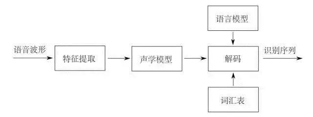
Speech recognition refers to the process of converting a segment of speech signal into corresponding text information. The system primarily consists of four main components: feature extraction, acoustic model, language model, and dictionary with decoding. To effectively extract features, it is often necessary to preprocess the collected audio signals by filtering and framing, extracting the signals to be analyzed from the raw signals. Subsequently, the feature extraction process transforms the audio signals from the time domain to the frequency domain, providing suitable feature vectors for the acoustic model. The acoustic model then calculates the scores of each feature vector based on their acoustic characteristics, while the language model computes the probabilities of possible word sequences corresponding to the audio signal based on linguistic theories. Finally, the dictionary is used to decode the word sequences, resulting in the final possible text representation.

Acoustic Signal Preprocessing

As a prerequisite and foundation for speech recognition, the preprocessing of speech signals is crucial. During the final template matching, the feature parameters of the input speech signal are compared with the feature parameters in the template library. Therefore, only by obtaining feature parameters that can characterize the essential features of the speech signal during the preprocessing stage can these parameters be matched for a high recognition rate.

First, the audio signal needs to be filtered and sampled, primarily to eliminate frequencies of non-human vocalization and interference from 50Hz electrical current. This process is generally accomplished using a bandpass filter, setting upper and lower cutoff frequencies, followed by quantization of the original discrete signals. Next, the high and low frequency segments of the signal need to be smoothed to facilitate solving the spectrum under the same signal-to-noise ratio conditions. The framing and windowing operation is aimed at ensuring the short-term stationary characteristics of the continuous signal by dividing it into independent frequency-stable segments for analysis, typically using pre-emphasis techniques. Finally, endpoint detection is necessary to correctly determine the start and end points of the input speech signal, primarily through short-term energy (the amplitude variation of the signal within the same frame) and short-term average zero-crossing rate (the number of times the sampled signal crosses zero within the same frame).

Acoustic Feature Extraction

After completing the signal preprocessing, the crucial operation of feature extraction follows. Simply recognizing the raw waveform does not yield good recognition results; features extracted after frequency domain transformation are used for recognition. The feature parameters used for speech recognition must meet the following criteria:

1. Feature parameters should describe the fundamental characteristics of speech as much as possible;

2. Minimize coupling between parameter components and compress the data;

3. The process of calculating feature parameters should be simplified to enhance algorithm efficiency. Pitch period, resonance peak values, and other parameters can serve as feature parameters representing speech characteristics.

Currently, the most commonly used feature parameters by mainstream research institutions are Linear Predictive Cepstral Coefficients (LPCC) and Mel Frequency Cepstral Coefficients (MFCC). Both feature parameters operate on speech signals in the cepstral domain, with the former using the vocal model as a starting point to derive cepstral coefficients using LPC technology. The latter simulates the auditory model, using the output of the speech filtered through a filter bank model as acoustic features, followed by transformation using Discrete Fourier Transform (DFT).

The pitch period refers to the vibration period of the vocal cords (fundamental frequency), which effectively characterizes the features of speech signals. Therefore, pitch period detection has been a critical research focus since the early studies on speech recognition. The resonance peak refers to areas of concentrated energy in the speech signal, representing the physical characteristics of the vocal tract and being a primary determinant of speech quality, making it another vital feature parameter. Additionally, many researchers have begun applying methods from deep learning to feature extraction, achieving rapid progress.

Acoustic Model

The acoustic model is a crucial component in speech recognition systems, and its ability to distinguish between different basic units directly impacts recognition results. Speech recognition is essentially a pattern recognition process, with the core of pattern recognition being the classifier and classification decision problem.

Typically, a dynamic time warping (DTW) classifier is effective for isolated word and small vocabulary recognition, providing good recognition results with fast recognition speed and low system overhead. However, in large vocabulary and speaker-independent speech recognition, the performance of DTW declines sharply. In such cases, using the Hidden Markov Model (HMM) for training significantly improves recognition results. Traditionally, continuous Gaussian Mixture Models (GMM) are used to characterize the state output density functions, hence the term GMM-HMM framework.

Moreover, with the advancement of deep learning, deep neural networks have been employed for acoustic modeling, forming the so-called DNN-HMM framework, which has also achieved excellent results in speech recognition.

Gaussian Mixture Model

For a random vector x, if its joint probability density function conforms to the formula, it is said to follow a Gaussian distribution, denoted as x ∼N(µ, Σ).

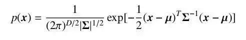
Where µ is the expectation of the distribution, and Σ is the covariance matrix of the distribution. Gaussian distribution has a strong capability to approximate real-world data and is easy to compute, making it widely used across various disciplines. However, many types of data cannot be adequately described by a single Gaussian distribution. In such cases, we can use a mixture of multiple Gaussian distributions to describe these data, where multiple components are responsible for different underlying data sources. At this point, the random variable conforms to the density function.

Where M is the number of components, usually determined by the scale of the problem.

The model used to describe data following a mixture of Gaussian distributions is called a Gaussian Mixture Model. Gaussian Mixture Models are widely used in the acoustic models of many speech recognition systems. Considering the relatively high dimensionality of vectors in speech recognition, we typically assume that the covariance matrix Σm in the mixture of Gaussian distributions is a diagonal matrix. This greatly reduces the number of parameters and enhances computational efficiency.

Using Gaussian Mixture Models to model short-term feature vectors has several advantages: first, Gaussian Mixture Models have strong modeling capabilities; as long as the total number of components is sufficiently large, they can approximate a probability distribution function with arbitrary precision. Additionally, using the EM algorithm allows the model to converge easily on training data. For issues like computational speed and overfitting, researchers have also developed parameter-tied GMMs and subspace Gaussian Mixture Models (subspace GMM) to address these concerns. Besides using the EM algorithm for maximum likelihood estimation, we can also train Gaussian Mixture Models using discriminative error functions directly related to word or phoneme error rates, significantly improving system performance. Therefore, until the emergence of deep neural network techniques in acoustic modeling, Gaussian Mixture Models remained the top choice for modeling short-term feature vectors.

However, Gaussian Mixture Models also have a significant drawback: their modeling capability is poor for data located near a nonlinear manifold in vector space. For example, if some data are distributed on either side of a sphere and are very close to the sphere’s surface, a suitable classification model may only require a few parameters to distinguish between the two sides. However, if we use a Gaussian Mixture Model to depict their actual distribution, we may need many Gaussian components to accurately characterize it. This drives us to seek a model that can utilize speech information more effectively for classification.

Hidden Markov Model

Now, consider a discrete random sequence. If the transition probabilities satisfy the Markov property, meaning that future states are independent of past states, it is called a Markov Chain. If the transition probabilities are time-invariant, it is termed a homogeneous Markov Chain. The outputs of a Markov Chain correspond one-to-one with predefined states, meaning that for any given state, the output is observable and has no randomness. If we expand the outputs to make each state of the Markov Chain output a probability distribution function, the states of the Markov Chain can no longer be directly observed, but can only be inferred from other variables that conform to probability distributions influenced by state changes. A model that uses this assumption of hidden Markov sequences to model data is called a Hidden Markov Model.

In the context of speech recognition systems, we use Hidden Markov Models to characterize the sub-state changes within a phoneme, addressing the correspondence between feature sequences and multiple basic speech units.

Using Hidden Markov Models in speech recognition tasks requires calculating the model’s likelihood over a segment of speech. During training, we need to use the Baum-Welch algorithm to learn the parameters of the Hidden Markov Model and perform maximum likelihood estimation (MLE). The Baum-Welch algorithm is a special case of the EM (Expectation-Maximization) algorithm, iteratively calculating conditional expectations in the E-step and maximizing conditional expectations in the M-step using forward and backward probability information.

Language Model

The language model primarily characterizes the habitual ways in which humans express language, emphasizing the intrinsic connections between words in terms of their arrangement structure. During the decoding process of speech recognition, the language model is referenced for inter-word transitions, and a good language model can not only improve decoding efficiency but also enhance recognition rates to some extent. Language models can be divided into rule-based models and statistical models, with statistical language models using probabilistic methods to depict the inherent statistical laws of language units. They are simple and practical in design and have achieved good results, being widely used in speech recognition, machine translation, sentiment recognition, and other fields.

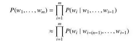
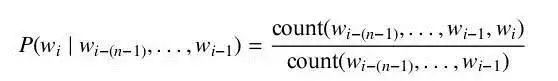
The simplest yet most commonly used language model is the N-gram Language Model. The N-gram model assumes that the probability of the current word, given the context, depends only on the preceding N-1 words. Thus, the probability of the word sequence w1, . . . , wm can be approximated as follows:

To obtain the probability of each word in the formula given its context, we need a sufficient amount of text in that language for estimation. This can be calculated directly using the proportion of word pairs in the context among all word pairs in the entire context.

For word pairs that do not appear in the text, we need to use smoothing methods for approximation, such as Good-Turing estimation or Kneser-Ney smoothing.

Decoding and Dictionary

The decoder is the core component of the recognition phase, decoding speech using trained models to obtain the most likely word sequences or generating recognition lattices for subsequent components to process. The core algorithm of the decoder is the dynamic programming algorithm Viterbi. Due to the enormous decoding space, we typically use a token passing method with limited search width in practical applications.

Traditional decoders dynamically generate the decoding graph entirely, such as HVite and HDecode in the well-known speech recognition toolkit HTK (HMM Tool Kit). This implementation occupies less memory; however, considering the complexity of various components, the entire system’s flow is cumbersome, making it inconvenient to efficiently combine language models and acoustic models, and more challenging to scale. Nowadays, mainstream decoder implementations partially use pre-generated finite state transducers (FST) as preloaded static decoding graphs. Here, we can construct the four parts: language model (G), vocabulary (L), context-related information (C), and Hidden Markov Model (H) as standard finite state transducers and combine them through standard finite state transducer operations to create a transducer from context-related phoneme sub-states to words. This implementation method uses additional memory space, but it tidies up the instruction sequence for the decoder, making it easier to construct an efficient decoder. Moreover, we can pre-optimize the pre-built finite state transducers, merging and trimming unnecessary parts to make the search space more reasonable.

Working Principle of Speech Recognition Technology

First, we know that sound is essentially a wave. Common formats like mp3 are compressed formats that must be converted into uncompressed pure waveform files for processing, such as Windows PCM files, commonly known as wav files. In addition to a file header, wav files store a series of points representing the sound waveform. Below is an example of a waveform.

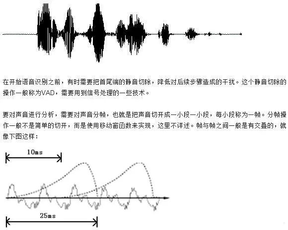
In the image, each frame is 25 milliseconds long, with a 15-millisecond overlap between two frames. This is referred to as framing with a length of 25ms and a shift of 10ms.

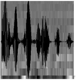
After framing, the speech is divided into many small segments. However, the waveform has almost no descriptive capability in the time domain, so it must be transformed. A common transformation method is to extract MFCC features, which convert each frame of waveform into a multidimensional vector based on the physiological characteristics of the human ear. This vector can be simply understood as containing the content information of that frame of speech. This process is called acoustic feature extraction.

At this point, the sound is represented as a matrix with 12 rows (assuming the acoustic features are 12-dimensional) and N columns, referred to as the observation sequence, where N is the total number of frames. The observation sequence is illustrated in the image below, where each frame is represented by a 12-dimensional vector, and the color depth of the blocks indicates the magnitude of the vector values.

Next, we need to introduce how to convert this matrix into text. First, we need to introduce two concepts:

Phoneme: The pronunciation of a word consists of phonemes. For English, a commonly used phoneme set is a set of 39 phonemes from Carnegie Mellon University. Chinese generally directly uses all initials and finals as the phoneme set, and additionally distinguishes between tones and non-tones, which will not be elaborated on here.

State: Here, it is sufficient to understand it as a more detailed unit of speech than a phoneme. Typically, a phoneme is divided into three states.

How does speech recognition work? In reality, it is not mysterious at all; it is merely:

Step one: Recognize frames as states.

Step two: Combine states into phonemes.

Step three: Combine phonemes into words.

As illustrated below:

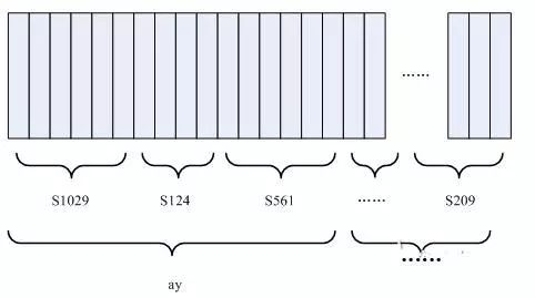
In the image, each small vertical bar represents a frame. Several frames of speech correspond to one state, three states combine into one phoneme, and several phonemes combine into one word. This means that as long as we know which state corresponds to each frame of speech, the recognition result will emerge.

So how do we determine which state corresponds to each frame? An intuitive approach is to check which state has the highest probability for a given frame, and that frame belongs to that state. For example, in the diagram below, this frame has the highest conditional probability in state S3, so we assume this frame belongs to state S3.

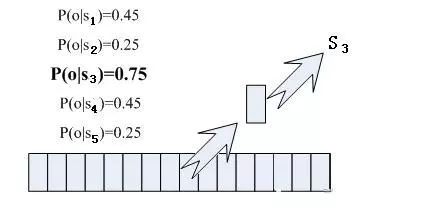
Where do the probabilities used come from? There is something called an “acoustic model” that contains a large number of parameters. Through these parameters, we can determine the probabilities corresponding to frames and states. The method to obtain this large set of parameters is called “training,” which requires a vast amount of speech data.

However, this approach has a problem: each frame will receive a state number, resulting in a disorganized set of state numbers for the entire speech. Adjacent frames will typically have different state numbers. For instance, if the speech has 1000 frames, and each frame corresponds to one state, then approximately 300 phonemes will be formed from every three states. However, this segment of speech does not actually contain that many phonemes. If we proceed this way, the resulting state numbers may not combine into phonemes at all. In reality, adjacent frames should logically have the same state most of the time due to their short duration.

A common method to resolve this issue is to use Hidden Markov Models (HMM). This concept may sound complex, but it is quite simple to use:

Step one: Build a state network.

Step two: Find the path in the state network that best matches the sound.

This confines the results within a pre-defined network, thus avoiding the issue mentioned earlier. However, it also introduces a limitation; for example, if your defined network only contains the state paths for “It’s sunny today” and “It’s raining today,” the recognized result will inevitably be one of these two sentences, regardless of what is actually spoken.

To recognize arbitrary text, you would need to make this network large enough to encompass the paths for any text. However, the larger the network, the more difficult it becomes to achieve reasonable recognition accuracy. Therefore, it is crucial to choose the network’s size and structure based on the actual task requirements.

Building the state network involves expanding from a word-level network to a phoneme network, and then to a state network. The speech recognition process essentially involves searching for the best path in the state network, with the probability of the speech corresponding to this path being maximized, a process known as “decoding.” The algorithm for path search is a dynamic programming pruning algorithm known as the Viterbi algorithm, used to find the globally optimal path.

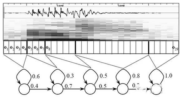
The cumulative probability mentioned here consists of three components:

Observation probability: The probability corresponding to each frame and each state.

Transition probability: The probability of each state transitioning to itself or to the next state.

Language probability: The probability derived from the statistical regularities of the language.

Among these, the first two probabilities are obtained from the acoustic model, while the last one is derived from the language model. The language model is trained using a large amount of text, utilizing the statistical regularities of a language to help improve recognition accuracy. The language model is essential; without it, when the state network is large, the recognized results can often be a jumble.

This essentially completes the speech recognition process, which is the working principle of speech recognition technology.

Workflow of Speech Recognition Technology

Generally, a complete speech recognition system works in seven steps:

1. Analyze and process the speech signal to remove redundant information.

2. Extract key information affecting speech recognition and feature information expressing language meaning.

3. Closely follow the feature information to recognize words at the smallest unit level.

4. Recognize words according to the grammar of different languages in the correct order.

5. Use contextual meaning as auxiliary recognition conditions, beneficial for analysis and recognition.

6. Based on semantic analysis, segment key information, retrieve recognized words, and connect them while adjusting sentence structure according to meaning.

7. Combine semantics to carefully analyze the interrelation of contexts and appropriately modify the current processing sentence.

The principles of speech recognition include three key points:

1. The encoding of linguistic information in speech signals is performed according to the time variation of the amplitude spectrum;

2. Since speech is readable, meaning that acoustic signals can be represented by multiple distinct, discrete symbols without considering the content conveyed by the speaker;

3. Speech interaction is a cognitive process, so it must not be separated from grammar, semantics, and usage norms.

Preprocessing includes sampling the speech signal, overcoming aliasing filtering, and eliminating noise influences caused by individual pronunciation differences and the environment. Additionally, it considers the selection of basic units for speech recognition and endpoint detection issues. Repeated training involves having speakers repeatedly produce speech to remove redundant information from raw speech signal samples, retaining key information, and organizing the data according to specific rules to form a pattern library. Pattern matching is the core part of the entire speech recognition system, determining the meaning of the input speech based on the similarity between input features and stored patterns.

Frontend processing first processes the raw speech signal, then performs feature extraction, eliminating noise and the influences of different speakers’ pronunciations, ensuring that the processed signals more completely reflect the essential features of speech.