Overview of Generative Adversarial Networks (GAN) in Graph Networks

Background Introduction

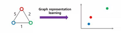
The main purpose of Graph Representation Learning (Graph Representation Learning, Network Embedding, Graph Embedding) is to map each node in the graph to a low-dimensional vector space, preserving the original structure and distance information of the graph. Intuitively, two points that are close together in the graph should also be close together in the low-dimensional space. As shown in the figure below (the numbers on the edges represent the lengths of the edges).

Research on graph representation learning has been ongoing for a long time, starting from the simplest adjacency matrix representation, to matrix decomposition (SVD) of the adjacency matrix, and then to the more popular random walk-based methods (DeepWalk, Node2Vec) in recent years, as well as the recent Graph Neural Network (GNN) and Graph Attention Network (GAT) models based on attention mechanisms. The goal is to map the network structure to a low-dimensional space for various tasks such as link prediction, node classification, etc.

This article mainly introduces the latest advancements of Generative Adversarial Networks (GAN) in graph representation learning. In this article, network models such as those in neural networks are referred to as models; network structures such as those in social networks are referred to as graph networks.

GraphGAN Model

The paper [1] categorizes methods for graph representation learning into two types: the first type is called generative models, and the second type is called discriminative models.

Generative models assume that each node has a latent probability distribution that reflects its connection to every other node. The main goal of generative models is to find a vector representation for the nodes in the graph network that closely approximates this latent probability distribution. In paper [1], this latent probability distribution is represented as Ptrue(V|Vc), where Vc represents the observed node, and Ptrue(V|Vc) refers to the probability of an edge existing between node V and Vc, excluding Vc.

Discriminative models directly learn the probability of an edge existing between two nodes. This method combines the two endpoints Vi and Vj of the edge as features, and outputs the probability P(|Vi, Vj) that the edge exists. Discriminative models are often supervised.

GraphGAN combines generative and discriminative models, consisting of two important components: the generator G(v|v_c ; θ_G) and the discriminator D(v|v_c ; θ_D). The generator maintains a vector for each node, and these vectors together form θG. G(v|v_c ; θ_G) indicates the probability that there is an edge between V and Vc given the node Vc and parameters θ_G. The purpose of G(v|v_c ; θ_G) is to learn and approximate the true distribution Ptrue(V|Vc). The discriminator also maintains a vector for each node, and these vectors together form θ_D. D(v|v_c ; θ_D) determines whether there is an edge between V and Vc based on the vector θ_D.

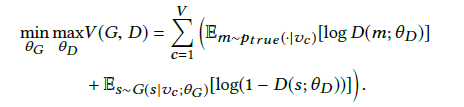
GraphGAN employs the common adversarial mechanism seen in GAN networks: the generator G tries to approximate Ptrue(V|Vc) as closely as possible to find nodes similar to the neighbors of Vc to deceive the discriminator D, while the discriminator D checks whether the given node V is a real neighbor of Vc or generated by the generator. The core of the GraphGAN method lies in the objective function in formula (1):

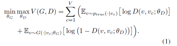
Given θ_D, the generator G aims to minimize the value of the following equation:

This means reducing the probability that (V, Vc) is judged by D as non-neighbors;

Given θ_G, the discriminator aims to maximize the value of the following equation:

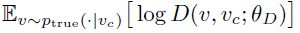
This means that the probability of judging real samples as neighbors should be as close to 1 as possible.

At the same time, maximize the value of the following equation:

This indicates that the probability of judging samples generated by the generator should be as close to 0 as possible.

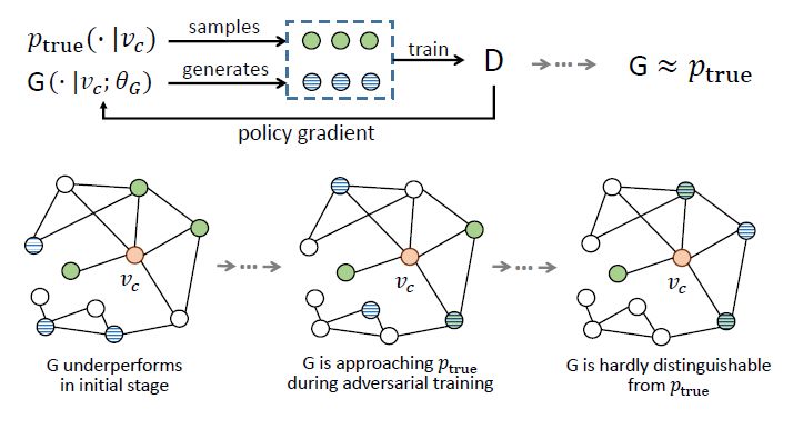
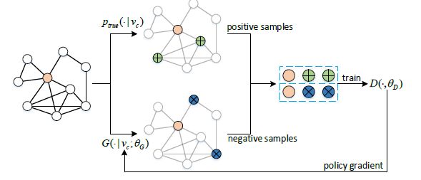
Understanding formula (1) essentially provides insight into the inner workings of GraphGAN. The figure below illustrates the workflow of GraphGAN. θ_D and θ_G can be iteratively updated through alternating minimization and maximization of the V(G,D) function. In each iteration, we sample some green points that are real neighbors of Vc from Ptrue, and generate some blue points that are close to Vc from G. We treat the green points as positive samples and the blue points as negative samples to train D. After obtaining D, we use the signals in D to train G through policy gradient. This process is repeated until the generator G and Ptrue are very close. Initially, G is relatively poor, so for a given Vc, the points sampled by G are far from Vc. As training continues, the sampled points will gradually approach Vc, and eventually, the points sampled by G will almost all become true neighbors of Vc, making G and Ptrue difficult to distinguish.

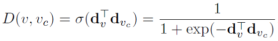
The implementation of the discriminator D is the inner product of the two node vectors followed by a sigmoid:

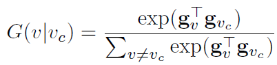
The basic implementation of the generator G is a softmax function, which selects the V closest to the Vc vector:

Another technical contribution of the paper is the design of a generation rule based on limited-width search, allowing the generator to find neighboring nodes without calculating every other node in the graph network. This optimization is somewhat loosely related to the GAN network concept and will not be detailed here.

This concludes the main ideas and model modifications of the GraphGAN model. GraphGAN is built to address the crucial question of whether there exists an edge between two nodes in graph networks, providing insights for subsequent GAN models in the field of graph networks. Code:

https://github.com/hwwang55/GraphGAN

CommunityGAN Model

The paper [2] introduces a method for overlapping community detection based on the GAN model, called CommunityGAN. In fact, based on the node representations generated by GraphGAN, communities in graph networks can also be obtained through clustering methods. However, the representations in GraphGAN only consider edge information, while community formation often requires tighter structures like cliques. Therefore, the basic idea of CommunityGAN shifts from determining whether there is an edge between two nodes to determining whether multiple nodes are pairwise connected to address the community detection problem. Below is a brief introduction to the CommunityGAN model.

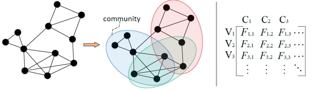
First, CommunityGAN assumes that each node can belong to multiple communities. The paper maintains a vector of community affiliation for each node, where each dimension of the vector represents the weight of the node belonging to the corresponding community, as shown in the figure below (V is the node id, C is the community id):

The paper first proves that in real graph networks, clique structures are more likely to appear within communities, meaning that nodes within the same community are more likely to be pairwise connected than nodes across communities. This aligns with our intuitive understanding. Based on this, CommunityGAN designs a model structure very similar to GraphGAN, with the only difference being that GraphGAN aims to determine whether there is an edge between two points, while CommunityGAN determines whether k points form a clique.

The generator G(s|v_c;θ_G) finds a set s given the node Vc, and considers s to form a clique where every node is connected. Assuming we target a triangle (3-clique), then |s|=2. The discriminator D(s,θ_D) determines whether the given set of nodes s forms a clique. With the background of GraphGAN, the objective function for CommunityGAN is easy to understand:

Where Ptrue is the distribution of real cliques in the network. Similar to GraphGAN, θ_G consists of the community affiliation vectors of each node, and θ_D is formed by combining the representation vectors of each node in the discriminator.

The model training is illustrated in the figure below: For each node Vc, we sample real clique structures from Ptrue as positive samples, and the generator finds nodes that are close in vector space based on θ_G to form negative samples to train the discriminator. Correspondingly, the discriminator scores the negative samples provided by the generator and feeds the scores back to the generator, which updates θ_G through policy gradient. The final community results are obtained by classifying nodes whose affiliation weights in θ_G exceed a certain threshold into the corresponding communities.

The logic for generating samples in CommunityGAN has also been optimized. By using random walks, it ensures that not all nodes need to be calculated in one selection. The paper places certain requirements on the initial state of θ_G, and the authors initialize θ_G using the AGM algorithm. In practical experiments, it was also found that when θ_G is not initialized properly, the CommunityGAN model is difficult to converge and may not learn at all. However, under reasonable initialization, CommunityGAN can significantly improve the quality of community division. Code:

https://github.com/SamJia/CommunityGAN

NetRA Model

To represent each node, the previous two models require sampling positive samples and generating negative samples for each node, which is challenging to implement on large networks in real life. The paper [3] adopts a graph representation model based on random walks. In fact, there are many graph representation models based on random walks, such as DeepWalk. However, these models have a problem: when we keep the number of samples constant, longer walks lead to worse performance. The reason is that as the length of the walk increases, the possible samples formed by the walks also increase, and when we sample insufficiently, overfitting occurs. Conversely, if we reduce the length of the walk, the ability to represent the network also decreases. The paper presents a series of experiments based on DeepWalk for edge prediction, assuming the average degree of nodes in the graph is d, the length of the walk is l, and the number of sampled walks is k. Their relationship is shown in the figure below.

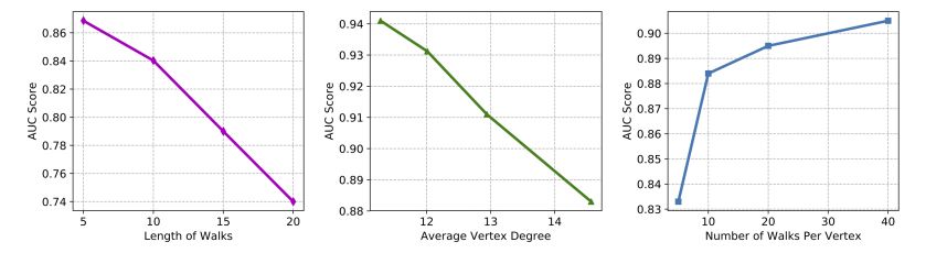
As shown in the figure above, when l or d increases, sampling becomes increasingly sparse, leading to overfitting and degraded performance. However, when we increase the number of walks, the model performance improves.

The NetRA model (Network Representation with Adversarially Regularized Autoencoders) proposed in paper [3] aims to avoid the overfitting problem of graph representation in sparse sampling situations. Specifically, NetRA introduces a regularization term from a GAN model to allow the encoder to extract more useful information. The overall framework of the NetRA model is shown in the figure below.

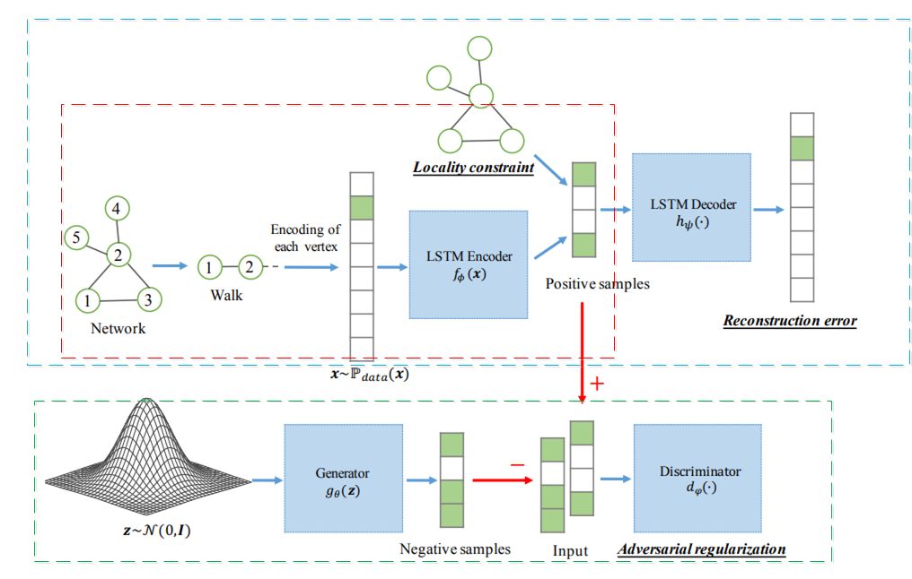
This model consists of three parts: Autoencoder (blue dashed box), GAN (green dashed box), and graph representation (red dashed box). Below is a brief introduction to each of these three parts.

Autoencoder

This part includes two functions, the encoding function fφ(·) and the decoding function h_Ψ(·). The encoding function maps the input to a low-dimensional space, while the decoding function can reconstruct the original input from the low-dimensional vector. The goal of the Autoencoder is to make the output after encoding and decoding as close as possible to the original input (x). Assuming Pdata is the true distribution of the data, the objective function of the Autoencoder is given by:

Here, the distance function is defined using cross-entropy as follows:

It is worth mentioning that this paper uses the LSTM model as the encoder, primarily because the LSTM model can effectively handle sequential inputs, allowing for the best representation of node sequences generated by random walks.

GAN

The green box in the figure represents the GAN model.

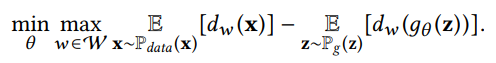
The generator g_θ(·) attempts to produce data that closely matches the true data distribution from noise, while the discriminator d_w(x) calculates the probability that the input x comes from real samples. Assuming the true sample distribution is Pdata(x) and the generator uses distribution Pg(z), then in the GAN model:

Here, the real samples are the low-dimensional vectors produced by the encoder in the Autoencoder above, so when we train the GAN, we also feed back the differences between positive and negative samples to the Encoder, allowing it to 1) extract more effective node representation information to distinguish fake samples; 2) avoid overfitting to prevent the generator from learning too easily.

Network Embedding

The Autoencoder samples paths from random walks in the network to obtain structural information about nodes, while the Network Embedding part retains edge information to gain local connection relationships between nodes. The embedding function remains the encoder from the Autoencoder, namely fφ(·). By minimizing the following function, the encoder ensures that the low-dimensional representations of connected nodes are close:

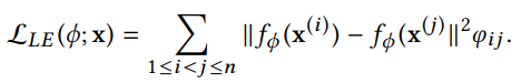
Here, φ_ij indicates whether there is an edge between nodes i and j, with 1 for an edge and 0 for no edge.

With the introduction of the three parts, the overall optimization function of the NetRA model can be expressed as:

Here, LAE represents the objective learned by the Autoencoder, while LLE and W are regularization terms for Network Embedding and the GAN model, ensuring that the encoder’s results preserve edge information from the network and prevent overfitting.

The training process of the NetRA model is as follows:

• Given a network, obtain some paths of length l through random walks. Construct feature sequences from the nodes in these paths using one-hot encoding and input them into the LSTM model to produce the Encoder’s output, i.e., the vector representation of the nodes.

• Input these vector representations into the Decoder function to obtain decoded feature vectors. Update the parameters of the Autoencoder by calculating the cross-entropy loss between these decoded feature vectors and the original feature vectors.

• Simultaneously, Network Embedding ensures that the encoding vectors of adjacent nodes are close to each other.

• Additionally, the encoded vectors are used as positive samples, and the vectors produced by the generator in the GAN model are used as negative samples to train the discriminator.

• The final node vector representation is the result produced by the encoder.

It can be seen that the NetRA model is not merely a GAN model structure; rather, it integrates the GAN model as part of a regularization term within the entire model to obtain node representations. This presents a different approach to applying GAN models.

Conclusion

This article introduced the basic methods of GAN models in graph representation learning (GraphGAN), their application in community detection (CommunityGAN), and the construction of more complex graph representation models (NetRA) using GAN as a regularization term. There is much ongoing research based on GAN models or adversarial learning ideas in graph representation learning; this article merely serves as an introduction to three common usage scenarios. Here is a compilation of papers related to graph neural networks, which have gained significant attention in the past two years.

In addition to close relationships such as classmates, colleagues, and family, we have also added many real estate agents, recruitment HRs, product distributors, and other non-close friends on WeChat. The edges between us and non-close friends are called weak ties. Our team has not only explored strong relationships in the relationship chain task but has also identified weak ties within the WeChat network.

References

[1] Wang etc. GraphGAN: Graph Representation Learning with Generative Adversarial Nets. AAAI’18.

[2] Jia etc. CommunityGAN: Community Detection with Generative Adversarial Nets. WWW’19.

[3] Yu etc. Learning Deep Network Representations with Adversarially Regularized Autoencoders. KDD’18.