Overview of Fisheye Camera Models in Computer Vision

Key Focus Areas of the Paper

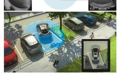
The surround-view fisheye camera is commonly used for close-range perception in autonomous driving, with four fisheye cameras around the vehicle covering a 360° range and capturing the entire close-range area. Some application scenarios include automatic parking, traffic congestion assistance, etc.

Since the primary focus of automotive perception is long-range sensing, there are limited datasets for close-range data, and research on related perception tasks is scarce. Compared to long-range perception, the high-precision object detection requirements at 10 centimeters and the local visibility of objects present additional challenges for surround-view perception. Moreover, due to the significant radial distortion of fisheye cameras, standard algorithms cannot easily be extended to surround-view use cases.

This paper aims to provide some references for researchers and engineering algorithm developers regarding automotive fisheye camera perception, including fisheye camera models and various perception tasks, and finally discusses common challenges and future research directions.

Application Background

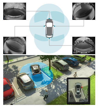
The surround-view system uses four sensors to form a network with overlapping areas, sufficient to cover the close-range area around the vehicle. The figure below shows the four views of a typical surround-view system and a representation of a typical parking scenario:

Wide-angle cameras with over 180 degrees are used for close-range perception, and any perception algorithm must consider the significant fisheye distortion inherent in such camera systems. This is a major challenge, as most work in the field of computer vision focuses on narrow field-of-view cameras with slight radial distortion. This paper primarily outlines panoramic cameras (e.g., image formation, configuration, and calibration), investigates existing technologies, and delves into the current challenges faced in the field.

Fisheye cameras present several significant challenges:

1. Exhibit strong radial distortion, reduced field of view, and distortion of surrounding features;
2. Greater deformation of objects, especially for nearby objects;
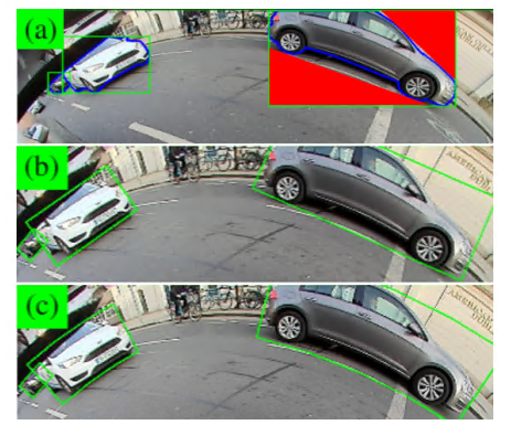
3. The algorithms using bounding boxes for object detection become more complex, as the boxes are difficult to optimally fit distorted targets, as shown in the figure below (although more complex representations that do not rely on rectangular boxes, such as using known radial distortion curve bounding boxes of fisheye cameras, are discussed in [14]):

For cameras without significant distortion, modeling is generally done using the pinhole model; however, fisheye cameras become complicated due to the lack of unified geometric structure, with many models using different characteristics to model fisheye cameras (the paper will elaborate in detail).

Fisheye Camera Models

This section will introduce several popular fisheye camera models, covering common solutions in the field as much as possible, guiding developers in selecting specific model types.

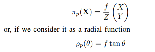
1. Pinhole Camera Model

The pinhole camera model is the standard projection function used in the fields of computer vision and robotics, with research limited to considering standard field-of-view cameras, modeled as:

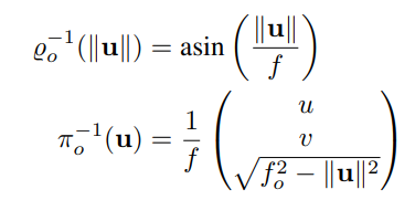
2. Classical Geometric Models

The models discussed in this section are referred to as classical models, which have been studied for at least sixty years [4]. The equisolid-angle model is also included, and references [27], [28] can be consulted, but no further elaboration will be provided here.

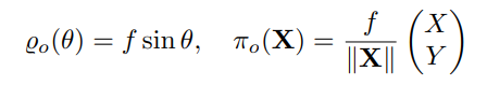
Equidistant Projection

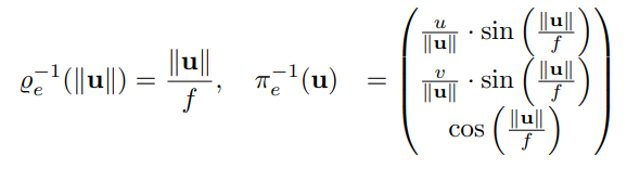
In the equidistant fisheye model, the projection radius Q_e(θ) is related to the field of view angle θ through simple scaling with the equidistant parameter f:

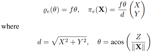
Inverse projection function:

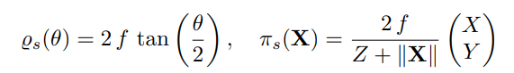
Stereographic Projection

Like the equidistant model, in stereographic projection, the projection center C is the projection center of the sphere (see figure 5b). Considering that the image plane has a tangent point along the Z-axis (optical axis), in stereographic projection, there exists a second center projection to the image plane, where the polar point of the tangent point forms the projection center, which is essentially a pinhole projection with a focal length of 2F.

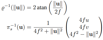
Inverse projection function:

Orthographic Projection

Similar to the previous projection models, orthographic projection starts from the projection to the sphere (see figure 5c), followed by an orthographic projection to the plane. Thus, orthographic projection is described as follows:

Inverse projection function:

Extended Orthographic Model

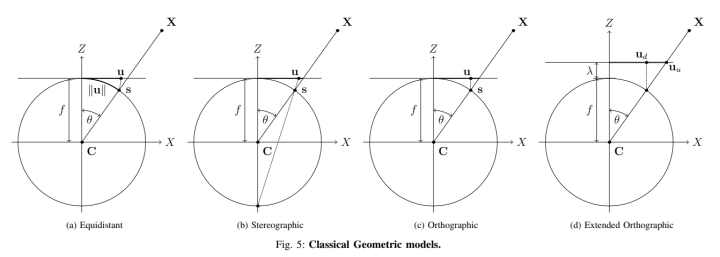
As shown in figure 5d, the extended orthographic model [29] extends the classical orthographic model by releasing the projection plane from the tangential position to the projection sphere, allowing an offset λ. In the case of converting the image from fisheye to planar image, this extension is used to control the size ratio between distorted and undistorted images. The distorted projection maintains the same form as the orthographic projection, however, the relationship between the distorted and undistorted radial distances and their inverses is given by:

This is a slightly simplified representation provided in [29], assuming f and (λ+f) are positive.

Extended Equidistant Model

The extended orthographic model is merely a transformation from projection to image mapping, and many models can be transformed into mapping on images in the same way as the extended orthographic model. Here, only an example of an equidistant model is given:

3. Algebraic Models

This briefly discusses the algebraic models of fisheye cameras, particularly polynomial models and the Division model. The discussion on polynomial models provides a complete introduction, although most of the other sections of this paper focus on geometric models.

Polynomial Model

The classic Brown-Conrady distortion model [31], [32] for non-fisheye cameras uses an odd polynomial to describe radial distortion on the image, where Pn represents some arbitrary Nth-order polynomial. To account for fisheye distortion, [18] proposed a polynomial fisheye transformation (PFET) image polynomial model. The difference between PFET and the Brown-Conrady model is that PFET allows both odd and even exponents to account for additional distortions encountered in fisheye cameras.

The MATLAB Computer Vision Toolbox [36] and NVIDIA’s DriveWorks SDK [37] include implementations of the polynomial-based fisheye model provided in [38]. In this case, polynomials are used to model both projections and non-projections without needing numerical methods to reverse the projection (which is the main computational issue of polynomial-based models).

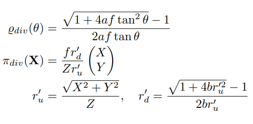
Division Model

The radial distortion Division model [17] has gained some popularity due to its good characteristics, at least for single-parameter variables, where straight lines project into circles [39]–[41], and for many lenses, single-parameter variables perform very well [42]. The model and its inverse are given by:

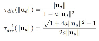
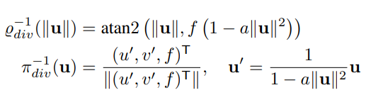
[30] extended this by adding an additional scaling parameter to improve modeling performance for certain types of fisheye lenses. Although the Division model was initially presented as an image mapping representation, it can be expressed as a projection function:

4. Spherical Models

Based on projections from points to a unit sphere (or its affine generalization), several newer fisheye models have also been considered over the past few decades.

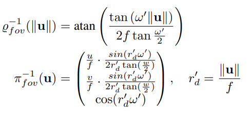
Field of View Model

The field of view model [19] and its inverse are defined as follows:

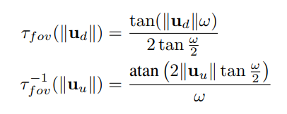
The parameter ω approximates the camera’s field of view, but not accurately [19]. This is an image model similar to the division model, where the projection function can be defined as:

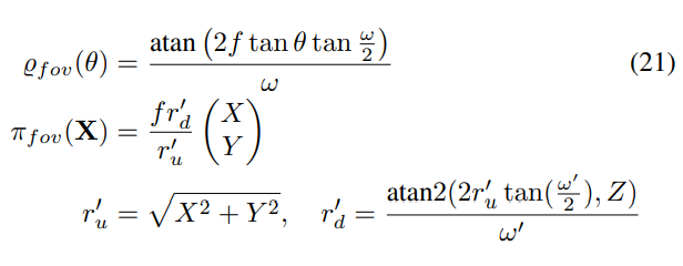
Inverse projection function:

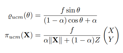
Unified Camera Model

The UCM was initially used to simulate reflective cameras [21], and later proved very useful in simulating fisheye cameras [43], [44]. It has been shown to perform well across a range of lenses [42], projecting points X onto a unit sphere and then onto the modeled pinhole camera (see figure 6a):

Inverse projection:

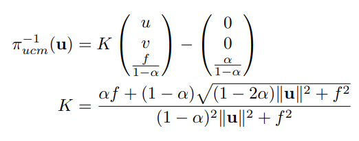
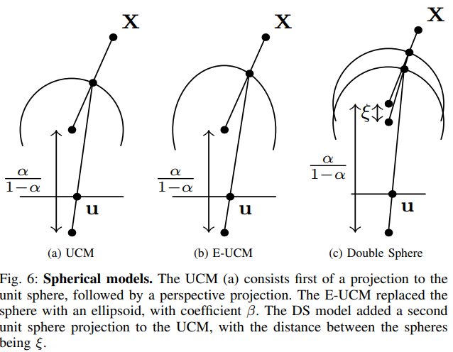
Enhanced Unified Camera Model

Based on UCM, the main extension is projecting spherical projections to ellipsoids (or, in fact, general quadratic surfaces), which can demonstrate certain accuracy gains, resulting in the E-UCM model:

Effective points and angles set:

Double Sphere Model

The UCM has also been extended by the Double Sphere (DS) model [23], which adds a second unit sphere projection to enable more complex modeling:

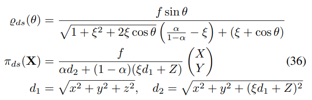
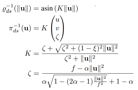
Inverse projection:

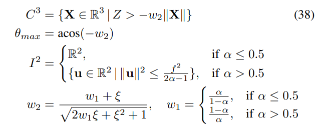
The effective range for projections and non-projections is:

5. Some Conclusions

Fisheye cameras have a large number of potential application models. This paper mentions 20 models, although it does not summarize all, yet it has been shown that there are strong relationships between many geometric models. At least seven models are related to general perspective projection or directly equivalent. Additionally, some recently developed fisheye models are mathematically equivalent to classic fisheye projection functions.

Panoramic Camera Systems

1. Visualization and System Arrangement

The main motivation for using fisheye cameras in SVC systems is to cover the entire 360° close-range area around the vehicle. This is achieved with four fisheye cameras, each having a horizontal field of view (hFOV) of about 190° and a vertical field of view (vFOV) of about 150°. Fisheye cameras have a very large angular volume coverage range, but their angular resolution is relatively low, making it difficult to perceive smaller objects at a distance. Therefore, they are primarily used as close-range perception sensors, whereas typical long-range front cameras have an hFOV of 120° and vFOV of 60°, with a significantly smaller angular volume but higher angular resolution allowing them to perceive distant objects. The large hFOV of fisheye cameras enables 360° coverage using only four fisheye cameras, and the large vertical field of view captures areas near the vehicle.

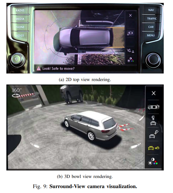
Generally, the four cameras are placed on the four sides of the car, marked with blue circles indicating their positions. The front camera is located on the front grille of the car, while the rear camera is usually located on the trunk door handle. The left and right cameras are positioned below the wing mirrors. Together, they cover the entire 360° area around the vehicle.

2. Calibration

Each model of the fisheye camera has a set of parameters (referred to as internal parameters) that must be completed through calibration. Additionally, there are external parameters of the camera, which are the position and orientation of the camera system in the vehicle’s coordinate system [57], [58]. The general calibration process involves first detecting image features (corners in the calibration board), followed by estimating internal and external parameters by minimizing the reprojection error of points.

Calibration in offline environments can be performed using OpenCV, OCamCalib [38], [60], [61], Kalibr [62]–[65], and [66] based on the extraction of chessboard features and correspondences between cameras, proposing a calibration process for multiple fisheye cameras on vehicles (internal and external parameters).

During the vehicle’s entire lifespan, the camera’s pose relative to the vehicle may drift due to wear of mechanical components. The camera system needs to use a class of algorithms to automatically update its calibration. To correct for changes in camera pose in online environments, photometric errors between the ground projections of adjacent cameras can be minimized [68]. The method by Choi et al. utilizes captured and detected corresponding lane markings from adjacent cameras to optimize initial calibration [69]. [70] Ouyang et al. proposed a strategy to optimize external orientation by estimating the vehicle odometry; these algorithms are primarily used to correct geometric misalignments but require an initial position obtained through offline calibration. Friel et al. [71] described a method for automatically extracting the essence of fisheye from automotive video sequences using a single-parameter fisheye model (such as the equidistant model).

3. Projection Geometry

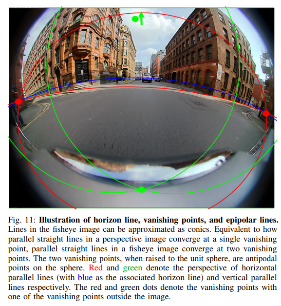
In pinhole cameras, any set of parallel lines on a plane converges at a vanishing point. In pinhole cameras, any set of parallel lines on a plane converges at a vanishing point. These parameters can be used to estimate internal and external parameters. For pinhole camera models, geometric problems can often be represented using linear algebra. In this case, the Hough transform can be used to detect parallel lines [72]. The set of all vanishing points is the horizon line of that plane. In real-world camera systems, pinhole cameras serve as a mathematical model of cameras, with errors manifesting in forms like optical distortion. This generally applies to narrow field-of-view cameras with small distortion. For wide field-of-view cameras, the distortion is too great to serve as a practical solution, and if the camera’s FOV exceeds 180°, there is no one-to-one relationship between points in the original image and the corrected image plane. For fisheye cameras, a better model is the spherical projection surface [73], [74]. In fisheye images, Hughes et al. [30] describe how these parallel lines can be approximated and fitted to determine the vanishing points or horizon lines for fisheye cameras. These parallel lines correspond to great circles on the sphere. Accordingly, the imaging of straight lines by fisheye cameras is approximated as cones [75], and the parallel lines captured by fisheye cameras converge at two vanishing points (as shown in the figure below).

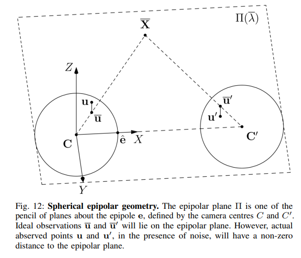
4. Spherical Epipolar Geometry

The geometric relationships of stereo vision are described by epipolar geometry, which can be used for subsequent depth estimation and SFM tasks. In the pinhole camera model, lines passing through the optical centers of two cameras define special points called epipoles, and this line is referred to as the baseline. Each plane through the baseline defines matching epipolar lines in the two image planes, where a point in one camera lies on the epipolar line in the other camera, and vice versa. This reduces the search for corresponding points in a stereo camera setup (stereo matching) to a 1D problem. For panoramic cameras, such as fisheye, using a spherical projection surface instead of a plane, a more intuitive approach is to discuss epipolar planes rather than epipolar lines, as shown in the figure below, where the ideal observations of a single 3D point by two cameras will lie on the same epipolar plane, just as they would lie on epipolar lines in the pinhole case.

5. Calibration

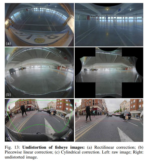
Common calibration methods for fisheye are shown in the figure below, where (a) shows standard line calibration, where loss of near information can be observed from the missing horizontal white line, and areas at the left and right edges are also lost. Although there is significant loss, this allows the use of standard camera algorithms. (b) shows a cube approximation, where the fisheye lens manifold surface is approximated by an open cube, which can be interpreted as a piecewise linear approximation of the fisheye projection surface. Each plane is a linear calibration, so standard algorithms can be used in each block.

However, the deformation on the two surfaces of the cube has significant distortion, making it difficult to detect targets split across two areas. Additionally, strong perspective distortion and blurring due to resampling artifacts at the periphery can be noted. In practice, a common correction process uses cylindrical surfaces, as shown in (c), which can be interpreted as a quasi-linear approximation since it is linear in the vertical direction and has quadratic curvature in the horizontal direction. The main advantage is that vertical objects remain vertical, as shown by the vertical lines on buildings [77]. Therefore, scan lines are preserved for horizontal searching stereo algorithms between two consecutive fisheye images (motion stereo) or between fisheye and narrow field-of-view cameras (asymmetric stereo). The main drawback is its inherent inability to capture the close-range area near the vehicle.

Fisheye Camera Perception Tasks

1. Semantic Tasks

Semantic Segmentation

The process of assigning category labels to each pixel in the image (such as pedestrians, roads, or curbs) is shown in the above figure (2nd column). Compared to the classic computer vision methods based on semantic segmentation used on front cameras, recent CNN-based methods have been very successful [78]. However, in urban traffic scenes, autonomous vehicles require a larger field of view to perceive the surrounding situation, especially at intersections. Deng et al. [79] proposed the Overlapping Pyramid Pooling Module (OPPNet), which generates various fisheye images and their respective annotations using multiple focal lengths. The OPP network is trained and evaluated on existing urban traffic scene semantic segmentation datasets for fisheye images. Additionally, to enhance the model’s generalization performance [79], a new scaling augmentation technique was proposed to enhance the dataset specifically designed for fisheye images.

A large number of experiments show that the scaling augmentation technique and OPP network perform well in urban traffic scenes. Saez et al. [80] introduced a real-time semantic segmentation technique, which is an adaptation of the Efficient Residual Factorization Network (ERFNet) [81] for fisheye road sequences, generating a new semantic segmentation dataset for fisheye cameras based on Cityscape [82]. Deng et al. [83] processed 360° road scene segmentation using surround-view cameras, as they are widely used in production vehicles. To address the distortion problem in fisheye images, a method called Restrained Deformable Convolution (RDC) was proposed. By learning the shape of convolution filters based on input feature maps, they allow effective geometric transformation modeling. Additionally, the authors proposed a magnification technique to convert perspective images into fisheye images, which helps create a large-scale training set for surround-view camera images. A semantic segmentation model based on RDC was also developed. A Multi-Task Learning (MTL) architecture is used to train real-world surround-view camera images by combining real-world and transformed images. These models were trained on the Cityscapes [82], FisheyeCityScapes [84], and SYNTHIA [85] datasets and tested on real fisheye images.

Object Detection

In fisheye images, object detection is most affected by radial distortion, as inherent distortion in fisheye image formation makes targets at different angles to the optical axis appear very different (as shown in the image below). Rectangular bounding boxes are often not the best representation of the target size, sometimes being half the size of the standard BB box, while the box itself is twice the size of the ROI object. Instance segmentation provides precise contours of objects, but the annotation cost is higher and also requires a BB estimation step.

FisheyeDet [87] emphasizes the need for useful datasets, creating simulated fisheye datasets by applying distortion to the Pascal VOC dataset [88]. Polygon representations and deformation shape matching assist FisheyeDet, and the paper proposes a Non-Prior Fisheye Representation Method (NPFRM) to extract adaptive distortion features without using lens patterns and calibration patterns. At the same time, a Deformation Shape Matching (DSM) strategy was proposed to achieve precise and robust positioning of targets in fisheye images.

SphereNet [89] and its variants [90]–[92] form CNNs on spheres and explicitly encode invariance to distortion. SphereNet achieves this by adjusting the sampling positions of convolution filters and wrapping them around the sphere. Existing perspective CNN models can be converted into omnidirectional scenes using SphereNet. Furthermore, quasi-distortion in the horizontal and vertical directions indicates that fisheye images do not conform to the spherical projection model. Yang et al. [93] compared the results of various detection algorithms that utilize equi-rectangular projection (ERP) sequences as direct input data, finding that CNNs only produce a certain accuracy without projecting ERP sequences onto normal 2D images.

FisheyeYOLO [14], [94] studied various representations such as oriented bounding boxes, ellipses, and general polygons. Using IoU metrics and precise instance segmentation ground truth, a new curved bbox method was proposed, improving the relative accuracy of the polygon bbox CNN model by 40.3%.

Perception Under Contamination

Panoramic cameras are directly exposed to the external environment and are prone to contamination. In contrast, front cameras are placed behind the windshield and are less likely to be affected. Generally, there are two types of contamination: opaque (mud, dust, snow) and transparent (water, oil, and grease). Due to limited visibility against the background, especially transparent dirt may be difficult to recognize, and contamination can significantly reduce perception accuracy. DirtyGAN [96] suggests using GANs to repair different stain patterns in real scenes. The boundaries of dirt are blurry and poorly defined, so manual annotations may have subjectivity and noise. Das et al. [97] proposed tile-level dirt classification to handle noisy annotations and improve computational efficiency.

From the perspective of perception, there are two ways to handle dirt. One method is to include robustness measures to improve perception algorithms. For example, Sakaridis et al. [99] proposed a fuzzy scene perception semantic segmentation. The other method is to recover contaminated areas. Mud or water droplets are typically static or occasionally exhibit low-frequency dynamics of moving droplets. Therefore, using video-based recovery techniques is more effective. Porav et al. [100] explored transparent dirt models by simulating raindrops on camera lenses using stereo cameras and dripping water sources. Uricar et al. [101] provided a benchmark for de-oiling datasets for surround-view cameras, using three cameras with varying degrees of dirt, while a fourth camera without dirt serves as the ground truth.

Geometric Tasks

Depth Estimation

Previous Structure from Motion (SfM) methods [106], [107] estimate inverse depth by parameterizing the disparity prediction of the network as non-projection operations during the view synthesis step. This parameterization is not applicable to fisheye cameras due to the significant distortion experienced, leading to angular differences on the epipolar curves compared to pinhole cameras. To adopt the same approach as pinholes, further calibration of fisheye images is required, but this would result in a loss of field of view.

Multi-view geometry principles applicable to pinhole models [108] are also applicable to fisheye images, estimating potential geometric structures by observing scenes from different viewpoints and establishing correspondences between them. It is noteworthy that when employing SfM methods, the norm values of CNN outputs are larger than the angular differences of fisheye cameras, as this makes it difficult to parameterize the angular differences into distances during view synthesis operations. Additionally, for fields of view greater than 180°, z values can be (close to) zero or negative, which can also lead to numerical issues in the model.

For LiDAR distance measurements, such as KITTI, depth prediction models can learn under supervision. Ravi Kumar et al. [109] adopted a similar approach, demonstrating the ability to predict distance maps for fisheye images trained using LiDAR ground truth. Nevertheless, LiDAR data is very sparse, and well-calibrated setups are very expensive. To overcome this issue, FisheyeDistanceNet [110] focuses on addressing one of the most challenging geometric problems, which is distance estimation for original fisheye cameras using image-based reconstruction techniques, a challenging task as the mapping from 2D images to 3D surfaces is a complex under-constrained problem.

Depth estimation is also an ill-posed problem since each pixel has several potential erroneous depths. UnRectDepthNet [16] introduces a general end-to-end self-supervised training framework for estimating monocular depth maps on original distorted images from different camera models. The authors showcase the results of the framework working on the original KITTI and WoodScape datasets.

SynDistNet [111] learns semantic-aware geometric representations that can eliminate photometric ambiguities in the self-supervised learning SfM context. The paper introduces a generalized robust loss function [112], which significantly enhances performance.

Visual Odometry

Liu et al. [114] describe traditional direct visual odometry techniques for fisheye stereo cameras. This technique simultaneously estimates camera motion and semi-dense reconstruction. The pipeline has two threads: one for tracking and one for mapping, with the paper using semi-dense direct image alignment in the tracking thread to estimate camera poses. To avoid epipolar issues, a planar scanning stereo algorithm is used for stereo matching and depth initialization.

Cui et al. [115] demonstrate a large-scale real-time dense geometric mapping technique using fisheye cameras. The camera pose is obtained from GNSS/INS systems, but they also propose that it can be retrieved from a visual inertial odometry (VIO) framework. Depth map fusion uses camera poses retrieved through these methods. Heng et al. [116] describe a semi-direct visual odometry algorithm for fisheye stereo cameras, where in the tracking thread, they track oriented patches when estimating camera poses; in the mapping thread, they estimate the coordinates and surface normals of each new patch to be tracked. In the techniques for detecting patch correspondences, descriptors or strong descriptor matching are not used; instead, the paper employs a method based on photometric consistency to find patch correspondences.

Various visual odometry methods for fisheye cameras include [117] and [118]. Additionally, Geppert et al. [117] extended visual inertial localization techniques in large-scale environments using a multi-camera visual inertial odometry framework, forming a system that allows for accurate drift-free pose estimation. Ravi Kumar et al. [119] used CNNs for visual odometry tasks, which act as an auxiliary task in a monocular distance estimation framework.

Motion Segmentation

Motion segmentation is defined as identifying independently moving objects (pixels) in a pair of sequences, such as vehicles and pedestrians, and separating them from the static background. MODNet [120] first explored this application scenario in autonomous driving, while InstanceMotSeg [121] defined and explored instance-level motion segmentation. FisheyeMODNet [122] extends this to fisheye cameras without requiring calibration and without explicit motion compensation. Mariotti et al. [74] completed this task using classic methods based on vehicle odometry [123]. They performed a spherical coordinate transformation for optical flow, applying height, depth, and epipolar constraints suitable for this setup, and the paper also proposed anti-parallel constraints to eliminate motion parallax blur, which often occurs when the car moves parallel to the ego vehicle.

Temporal Tasks

While geometric tasks such as depth and motion can be trained and inferred using multiple frames, outputs are defined only on a single frame. We define Temporal Tasks as tasks that output across multiple frames, which typically require sequential labeling across multiple frames.

Tracking

Object tracking is a common task that must associate objects across multiple frames. [124] discusses motion object detection and tracking for surround-view cameras, using classic optical flow-based methods for tracking. WEPDTOF [125] is a recently released dataset for pedestrian detection and tracking using fisheye cameras in elevated monitoring devices. Trajectory prediction is closely related to tracking, especially in 3D bird’s-eye view space in autonomous driving scenarios. The PLOP algorithm [126] explores vehicle trajectory prediction on fisheye front cameras after applying cylindrical correction.

Re-identification

Re-identification (Re ID) is the association of objects detected across cameras, which can also include temporal associations across cameras. Wu et al. [127] suggested implementing vehicle recognition on panoramic cameras and highlighted two significant challenges: first, due to fisheye distortion, occlusion, truncation, and other factors, it is difficult to detect the same vehicle from previous image frames in a single camera view. Secondly, the appearance of the same vehicle can change significantly depending on the camera used under multi-camera perspectives. The paper provides a new quality assessment mechanism to offset the effects of tracking box drift and target consistency (primarily employing attention-based Re ID networks, then pairing with spatial constraint methods to enhance performance across different cameras).

SLAM

FisheyeSuperpoint [132] introduces a unique training and evaluation method for fisheye images. As a starting point, SuperPoint [133], a self-supervised keypoint detector and descriptor, is employed to generate state-of-the-art homography prediction results. The paper proposes a fisheye adaptive framework for training on undistorted fisheye images, where fisheye distortion is used for self-supervised training of fisheye images. By projecting onto the unit sphere’s intermediate projection phase, fisheye images are transformed into new distorted images. The camera’s virtual pose can change in 6-Dof. Tripathi et al. [134] explore the issue of repositioning using surround-view fisheye cameras within ORB SLAM pipelines.

Multi-task Models

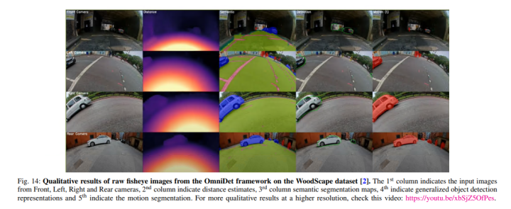
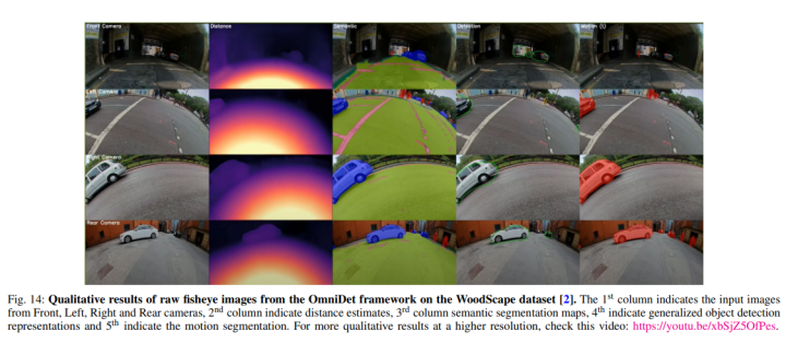
Feature extraction for multiple tasks using the same backbone is discussed for fisheye cameras, with Sistu et al. [147] proposing a joint MTL model for learning object detection and semantic segmentation. The primary goal is to achieve real-time performance on low-power embedded systems on-chip, with both tasks using the same encoder, where object detection employs a YOLO v2 decoder, while semantic segmentation uses an FCN8 decoder. Leang et al. explore different task weighting methods for two-task setups on fisheye cameras [148]. FisheyeMultiNet [149] discusses the design and implementation of an automatic parking system from the perspective of camera-based deep learning algorithms. On low-power embedded systems, FisheyeMultiNet is a real-time multi-task deep learning network capable of identifying all targets required for parking. The device is a four-camera system operating at 15fps while performing three tasks: object detection, semantic segmentation, and contamination detection. OmniDet [119] introduces an overall real-time scene understanding structure for close-range perception of the environment using only cameras, learning geometry, semantics, motion, localization, and contamination multi-tasks from a single deep learning model at a speed of 60 frames per second.

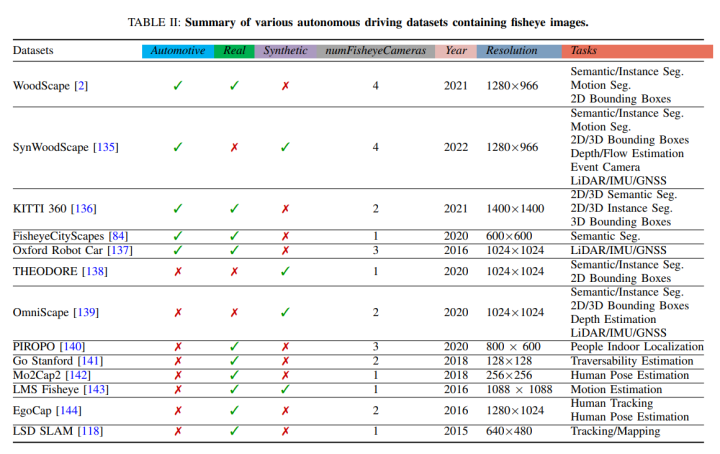
Fisheye Open Source Datasets

Fisheye-related datasets are shown in the figure below, involving tasks such as semantic segmentation, instance segmentation, 2D/3D detection, depth estimation, optical flow, localization, and tracking!!!!

Future Research Directions

The paper mainly focuses on distortion-aware CNNs, handling time variations, BEV perception, multi-camera models, unified modeling of close-range and long-range cameras, etc. For details, please refer to the proposed references.

References

[1] Surround-view Fisheye Camera Perception for Automated Driving: Overview, Survey & Challenges