Overview of CNN Convolution Methods

Important content delivered at the first time

• The Essence of Convolution

• Conventional Convolution

• Single-channel Convolution

• Multi-channel Convolution

• 3D Convolution

• Transposed Convolution

• 1×1 Convolution

• Depthwise Separable Convolution

• Dilated Convolution

Before introducing various convolutions, it is necessary to revisit the true meaning of convolution, looking at what convolution really is from the perspective of mathematics and image processing applications. Most deep learning tutorials rarely elaborate on the meaning of convolution; most only explain the convolution operation on images. As a result, many people are not very clear about the mathematical and physical significance of convolution, specifically why it is designed this way and the reasons behind this design.

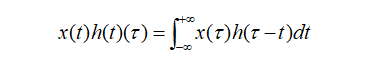
Tracing back to the mathematics textbook, convolution is also known as convolution or folding in functional analysis, and it is a mathematical operator generated by two functions x(t) and h(t). Its calculation formula is as follows:

Continuous form:

Discrete form:

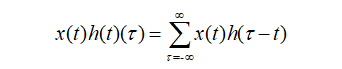
The formula is clear: the convolution of two functions is to first reverse one function (Reverse) and then perform a shift (Shift), which is the meaning of “卷” (roll). The “积” (product) means multiplying and summing the corresponding elements of the two shifted functions. Therefore, convolution is essentially a Reverse-Shift-Weighted Summation operation.

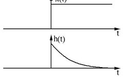
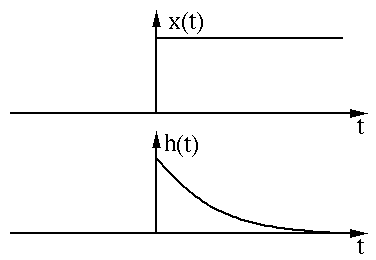
Numbers are less intuitive when invisible. We use the graphs of two functions to intuitively display the convolution process and meaning. The graphs of the two functions x(t) and h(t) are shown below:

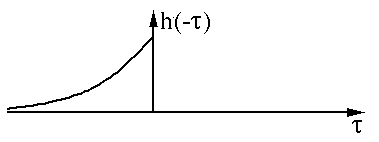
First, we perform the reverse (Reverse) operation on one of the functions h(t):

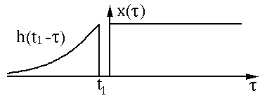
Then perform the shift (Shift):

The above process is the “卷” (roll). Then comes the “积” (product) process; since it is a continuous function, the multiplication and summation is in the form of integration, and the green part in the figure is the multiplication and summation part.

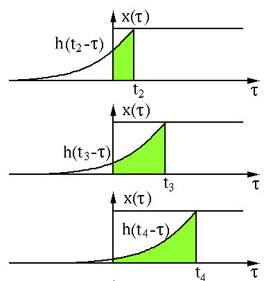
Image source:

http://fourier.eng.hmc.edu/e161/lectures/convolution/index.html

So why use convolution? Isn’t direct element multiplication good enough? In terms of image convolution operations, the author believes that convolution can better extract regional features, and using convolution kernels of different sizes can extract features at various scales of the image. Convolution has wide applications in signal processing, image processing, and other fields. Of course, in terms of deep learning, convolutional neural networks are mainly used in the field of images. After reviewing the essence of convolution, let’s systematically organize the typical convolution operations in CNN.

We start from the most primitive image convolution operation. Since images can have single-channel images (grayscale) and multi-channel images (RGB), the conventional convolution method can be divided into single-channel convolution and multi-channel convolution. There is not much difference between the two; it is just that convolution needs to be performed on each channel. Let’s first look at single-channel convolution.

In single-channel convolution, for the pixel matrix of the image, the convolution operation is to use a convolution kernel to scan the pixel matrix row by row and column by column, multiplying with the pixel matrix element-wise to obtain a new pixel matrix. The convolution kernel is also called a filter, and the area that the filter sweeps over the input pixel matrix is called the receptive field. Assuming the input image dimension is n*n*c, the filter dimension is f*f*n, the convolution stride is s, and the padding size is p, then the output dimension can be calculated as:

A standard single-channel convolution is shown in the figure below:

Image source:

https://towardsdatascience.com/intuitively-understanding-convolutions-for-deep-learning-1f6f42faee1

Here, we have not included padding and stride and other convolution factors, just to illustrate the general convolution process. So how do we understand multi-channel (3-channel) convolution? It’s actually quite simple. For example, if we have a 5*5*3 RGB 3-channel image, we can think of it as a stack of 3 5*5 images, and we can use 3 filters corresponding to the original single-channel filter to perform convolution on the three images. The convolved feature maps are then summed to produce the final result. Here, it is emphasized that the number of channels in the filter must match the number of channels in the input image; otherwise, some channels will be missed and not convolved. Now we use a 3*3*3 filter to convolve with a 5*5*3 input, and the output dimension will be 3*3. Here, the number of channels is reduced, so generally, we will use multiple 3-channel filters to perform convolution. Assuming we have used ten 3*3*3 filters, the final output will be 3*3*10, with the number of filters becoming the number of output feature map channels.

Image source:

https://towardsdatascience.com/a-comprehensive-introduction-to-different-types-of-convolutions-in-deep-learning-669281e58215

We can also understand multi-channel convolution from a 3D perspective: we can imagine a 3*3*3 filter as a three-dimensional cube. To compute the convolution operation of the cube filter on the input image, we first place the three-dimensional filter in the upper left corner, allowing the 27 numbers of the filter to multiply the pixel data in the red, green, and blue channels, respectively. The first nine numbers of the filter multiply the data in the red channel, the middle nine numbers multiply the data in the green channel, and the last nine numbers multiply the data in the blue channel. Summing these data gives the value of the first output pixel. The schematic is shown below:

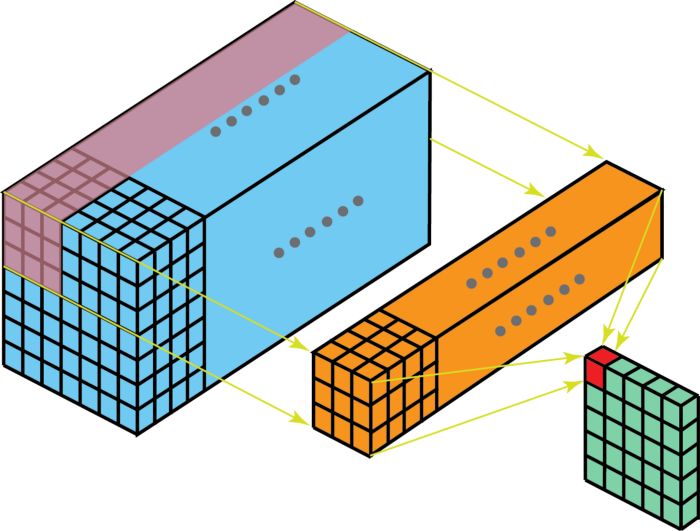
Image source:

https://towardsdatascience.com/a-comprehensive-introduction-to-different-types-of-convolutions-in-deep-learning-669281e58215

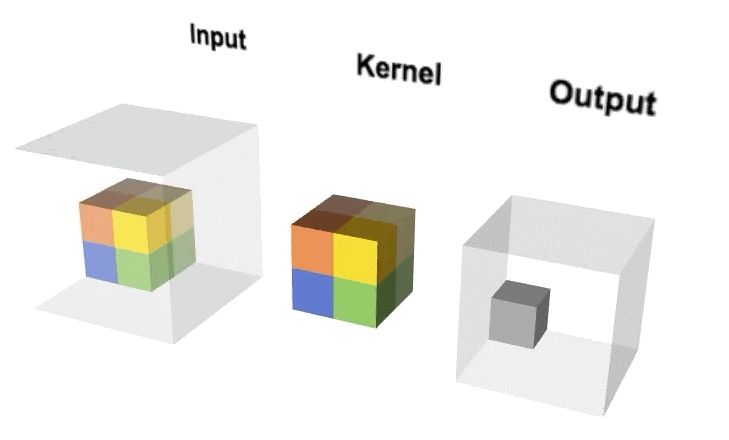
3D convolution can be extended by adding a depth dimension to 2D convolution. The input image is three-dimensional, the filter is also three-dimensional, and the corresponding convolution output is likewise three-dimensional. The operation schematic is shown below:

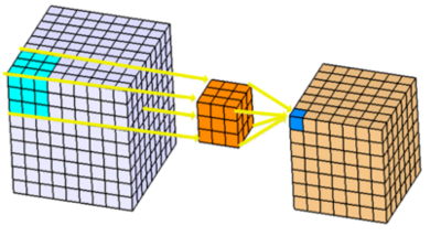
Imagine the dynamic diagram of 3D convolution. Using a 2*2*2 3D filter on a 4*4*4 input image for 3D convolution can yield a 3*3*3 output.

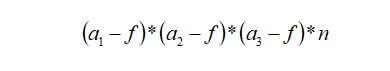
We can extend the calculation output formula of 2D convolution to derive the output dimension calculation formula for 3D convolution. Assuming the input image size is a1*a2*a3, the number of channels is c, the filter size is f*f*f*c, and the number of filters is n, then the output dimension can be expressed as:

3D convolution has a wide range of applications in medical imaging data, video classification, and more. Compared to 2D convolution, one feature of 3D convolution is that the computational load is immense, requiring relatively high computational resources.

Transposed convolution (also called deconvolution) is sometimes inaccurately referred to as inverse convolution. As we know, in conventional convolution, the size of the convolution feature map we obtain each time becomes smaller. However, in fields such as image segmentation, we need to gradually restore the size of the input. If we refer to the feature map becoming smaller during conventional convolution as downsampling, then the operation to restore resolution through transposed convolution can be called upsampling.

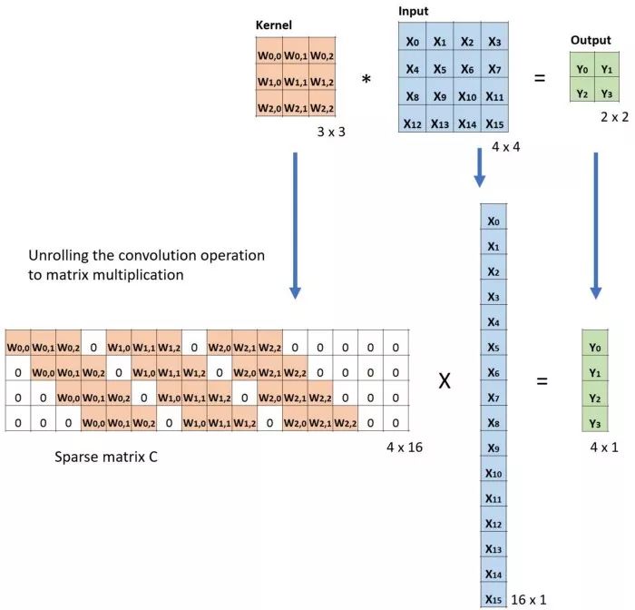
Essentially, transposed convolution is not different from conventional convolution. The difference lies in first padding the input size by a certain proportion to enlarge it, then transposing the convolution kernel used in conventional convolution, and finally performing convolution using the conventional convolution method, which constitutes transposed convolution. Assuming the input image matrix is X, the convolution kernel matrix is C, and the output of conventional convolution is Y, then:

Multiplying both sides by the transpose of the convolution kernel CT gives this formula, which is the input-output calculation of transposed convolution.

Assuming the input size is 4*4, the filter size is 3*3, the output of conventional convolution is 2*2, to demonstrate transposed convolution, we will sparsify the filter matrix to 4*16 and flatten the input matrix to 16*1, resulting in the corresponding output also being flattened to 4*1, as illustrated below:

Then, according to the method of transposed convolution, we transpose the convolution kernel matrix and verify using X=CTY:

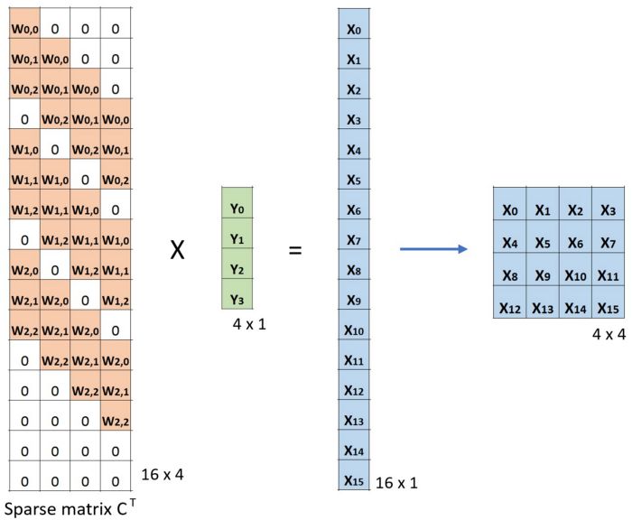
Image source:

https://towardsdatascience.com/intuitively-understanding-convolutions-for-deep-learning-1f6f42faee1

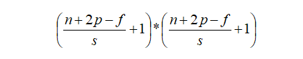
The last question about transposed convolution is the calculation of input-output sizes. We can derive the conversion formula for transposed convolution by transforming the conventional convolution calculation formula:

The first formula is the conversion formula for conventional convolution mentioned above, and the second formula is the input-output conversion formula for transposed convolution. Here, s is the stride of conventional convolution, p is the padding of conventional convolution, and f is the filter size. Although the formula derivation is simple, considering that (w2+2p-f)/s is likely to be indivisible, the conversion relationship between conventional convolution and transposed convolution needs to be divided into two cases.

The first case is when it can be directly divided. That is, when (w2+2p-f)%s=0, the conversion relationship between conventional convolution and transposed convolution. We compare a group of animations of conventional convolution and transposed convolution without padding conditions:

Conventional Convolution

Transposed Convolution

Image source:

https://github.com/vdumoulin/conv_arithmetic

In the above conventional convolution, the input is 2*2, and the filter is 3*3. According to the first formula above, the output is (4+2*0-3)/1 + 1=2, which can be divided, so the output is 2*2. Correspondingly, in transposed convolution: 1*(2-1)+3-2*0=4, indicating that the output of transposed convolution is 4*4.

The second case is a bit more complicated, which is the indivisible case. The indivisible case in conventional convolution is also called odd convolution. That is, when (w2+2p-f)%s!=0, how to establish the conversion relationship between conventional convolution and transposed convolution. In odd convolution, when encountering indivisible cases, we will perform rounding operations, so sometimes a small portion of pixels are neglected during convolution in conventional convolution, which needs to be added back during transposed convolution. We will illustrate this with a group of odd convolution examples.

Odd Conventional Convolution

Odd Transposed Convolution

Image source:

https://github.com/vdumoulin/conv_arithmetic

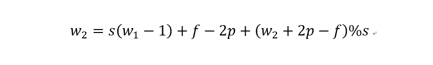
As shown in the above diagram, in odd conventional convolution, we convolve a 3*3 filter with a 6*6 input, padding=1, stride=2. According to the formula (6+2*1-3)/2, we find that it cannot be divided, so we round it to 3, and the output feature map size is 3*3. Because of the rounding operation, you can see that the rightmost column and the bottom row of padding are not included in the convolution calculation. This portion of data, which is neglected due to rounding, needs to be added back during transposed convolution. Therefore, the conversion formula for input-output in transposed convolution can be modified as follows:

In the above diagram, the input size is 3*3, the filter size is also 3*3, the padding is 1, but here the stride equals 2. Some students may ask why the convolution kernel only moves one step but the stride is 2? The kernel indeed only moves one step, but you can notice that we inserted many white blocks (zeros) into the input. Thus, from the current element value to the next element value, it actually moves through two strides. Therefore, the output size is 2*(3-1)+3-2*1+1=6. This is transposed convolution.

The great invention of 1×1 convolution comes from GoogLeNet’s inception v1 in 2014, primarily serving the purpose of dimensionality reduction to save computational costs. The 1×1 convolution has no difference in convolution method compared to conventional convolution; its main difference lies in its application scenarios and functions.

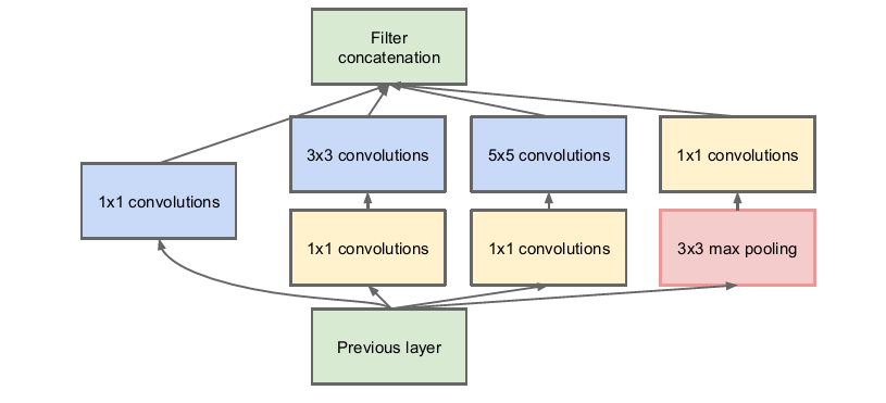
Inception v1 module

Next, let’s see what effects 1×1 convolution has. Suppose we currently have an input of 28*28*192, using 32 filters of size 5*5*192 to perform convolution, the output is 28*28*32, which seems unremarkable. Let’s take a look at its computational load; for each element value in the output, we need to perform 5*5*192 calculations, so the computational load for this convolution is: 28*28*32*5*5*192=120422400. The computational load of 5*5 convolution directly exceeds 100 million.

Now let’s see how 1×1 convolution performs. First, we use 16 filters of size 1*1*192 to convolve the input, resulting in an output size of 28*28*16. Then we convolve with 32 filters of size 5*5*16, resulting in an output of 28*28*32. After two convolutions, we still get an output of 28*28*32; let’s see the computational load. The computational load for the first convolution: 28*28*16*192=2408448, and for the second convolution: 28*28*32*5*5*16=10035200. The total computational load is about 1200000, which is a reduction of 10 times compared to the direct 5*5 convolution, significantly saving computational costs while ensuring network performance. This is the essence of 1×1 convolution.

From a dimensional perspective, convolution kernels can be viewed as a combination of spatial dimensions (width and height) and channel dimensions, while the convolution operation can be seen as a joint mapping of spatial correlation and channel correlation. From the 1×1 convolution in inception, it is possible to decouple spatial correlation and channel correlation in convolution, which may yield better results.

Depthwise separable convolution is an innovation based on 1×1 convolution. It mainly consists of two parts: depthwise convolution and 1×1 convolution. The purpose of depthwise convolution is to use a separate convolution kernel for each input channel, meaning that the channels are separated and then combined. The purpose of 1×1 convolution is to enhance depth. Let’s look at an example of depthwise separable convolution.

Suppose we use 128 filters of size 3*3*3 to convolve with an input of size 7*7*3, yielding an output of size 5*5*128. As shown in the figure below:

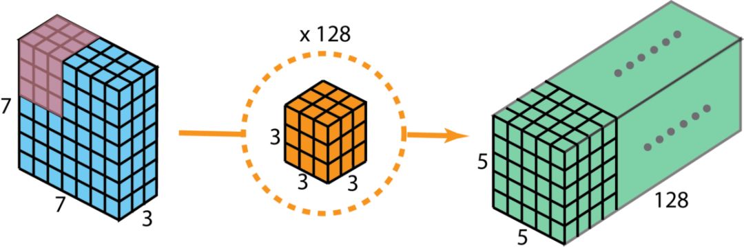
Image source:

https://towardsdatascience.com/intuitively-understanding-convolutions-for-deep-learning-1f6f42faee1

The computational load is 5*5*128*3*3*3=86400.

Now let’s see how to achieve the same result using depthwise separable convolution. The first step of depthwise separable convolution is depthwise convolution. Here, depthwise convolution means using three 3*3*1 filters to convolve the three channels of the input separately, resulting in three convolutions, each yielding a 5*5*1 output, which are then combined to produce a 5*5*3 output.

Now, to expand the depth to 128, we need to perform the second step of depthwise separable convolution: 1×1 convolution. We now use 128 filters of size 1*1*3 to convolve the 5*5*3 output, yielding a 5*5*128 output. The complete process is illustrated in the figure below:

Image source:

https://towardsdatascience.com/intuitively-understanding-convolutions-for-deep-learning-1f6f42faee1

Now let’s look at the computational load of depthwise separable convolution. The computational load for the first step, depthwise convolution: 5*5*1*3*3*1*3=675. The computational load for the second step, 1×1 convolution: 5*5*128*1*1*3=9600, totaling a computational load of 10275. It is evident that depthwise separable convolution saves 12 times the computational cost compared to conventional convolution while achieving the same convolution output.

Typical network models that apply depthwise separable convolution include Xception and MobileNet. Essentially, Xception is an inception network that applies depthwise separable convolution.

Dilated convolution, also known as atrous convolution or expansion convolution, simply adds some spaces (zeros) between the elements of the convolution kernel to expand the convolution kernel’s process. We use a dilation rate a to represent the degree of expansion of the convolution kernel. For example, when a=1,2,4, the receptive fields of the convolution kernel are shown in the figure below:

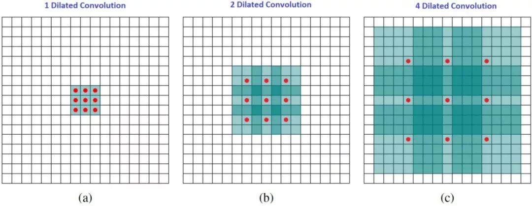
Image source:

https://towardsdatascience.com/intuitively-understanding-convolutions-for-deep-learning-1f6f42faee1

The relationship between the actual size of the convolution kernel after adding dilation and the original convolution kernel size is:

Where k is the original convolution kernel size, a is the dilation rate, and K is the actual convolution kernel size after dilation. In addition, the convolution method of dilated convolution is the same as that of conventional convolution. The dynamic schematic of dilated convolution when a=2 is shown below:

Image source:

https://github.com/vdumoulin/conv_arithmetic

What are the benefits of dilated convolution? One direct effect is that it can expand the receptive field of convolution. Dilated convolution can obtain a larger receptive field to gather more information at virtually no cost, which helps improve accuracy in detection and segmentation tasks. Another advantage of dilated convolution is that it can capture multi-scale contextual information. When we use different dilation rates for convolution kernel stacking, the receptive fields obtained become diverse and rich.

Group Chat

Welcome to join the reader group of the public account to exchange ideas with peers. Currently, there are WeChat groups for SLAM, 3D Vision, Sensors, Autonomous Driving, Computational Photography , Detection, Segmentation, Recognition, Medical Imaging, GAN, Algorithm Competitions (which will gradually be subdivided in the future), please scan the WeChat ID below to join the group, and note: “nickname + school/company + research direction”, for example: “Zhang San + Shanghai Jiao Tong University + Vision SLAM”. Please follow the format for notes, otherwise, you will not be approved. After successful addition, you will be invited to the relevant WeChat group according to your research direction. Please do not send advertisements in the group, otherwise, you will be removed from the group. Thank you for your understanding~