Click the above“Beginner’s Guide to Vision”, select to add “Bookmark” or “Pin”

[Guide] The latest 3D visualization tool ‘mm’ released by the Pytorch team can simulate matrix multiplication in a virtual world.
The simulated world of matrices is truly here.

Matrix multiplication (matmul) is a very important operation in machine learning, especially playing a key role in neural networks.
In a recent article by the Pytorch team, they introduced “mm”, a visualization tool for matmuls and combinations of matmuls.

By utilizing three spatial dimensions, ‘mm’ helps to build intuition and inspire ideas, especially suitable (but not limited to) for visual/spatial thinkers.
NVIDIA Senior Scientist Jim Fan stated, “Enter the neural network ‘matrix’.”
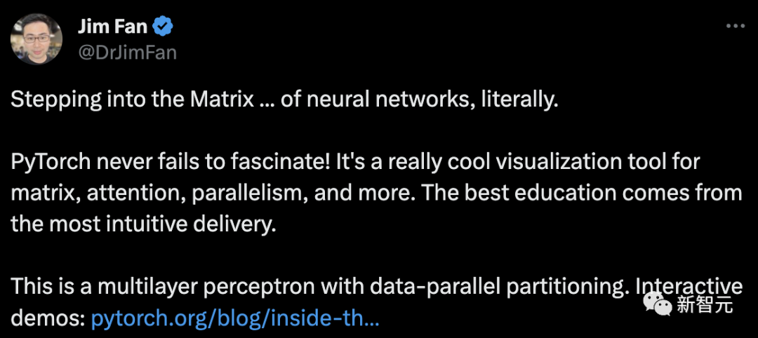
This is a very cool visualization tool for matrices, attention, parallelism, etc. The best education comes from the most intuitive delivery. This is a multi-layer perceptron with data parallel segmentation capability.
With three dimensions forming matrix multiplication, combined with the ability to load trained weights, you can visualize large composite expressions like attention heads and observe their actual performance.
The ‘mm’ tool is interactive, can run in a browser or notebook iframe, and retains its full state in the URL, allowing sharing of dialogue links.
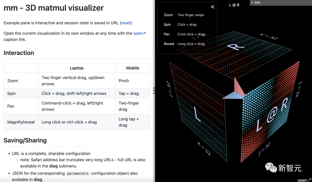
Address: https://bhosmer.github.io/mm/ref.html
Below, the reference guide provided by Pytorch introduces all available features of ‘mm’.
The research team will first introduce visualization methods to build intuition through visualizing some simple matrix multiplications and expressions, then delve into more examples.
Why is this visualization method better?
The visualization method of ‘mm’ is based on the premise that matrix multiplication is fundamentally a three-dimensional operation.
In other words:
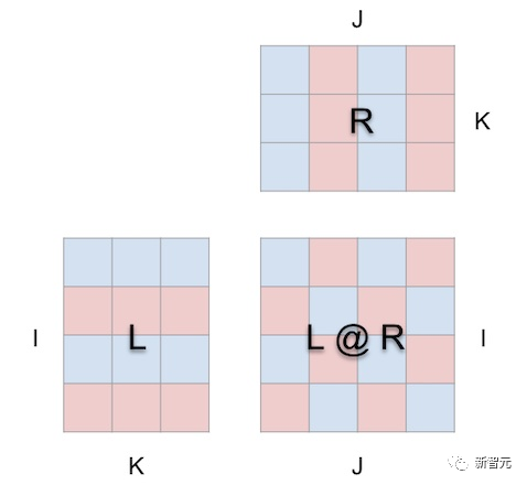
It is a piece of paper, which looks like this when opened with ‘mm’:
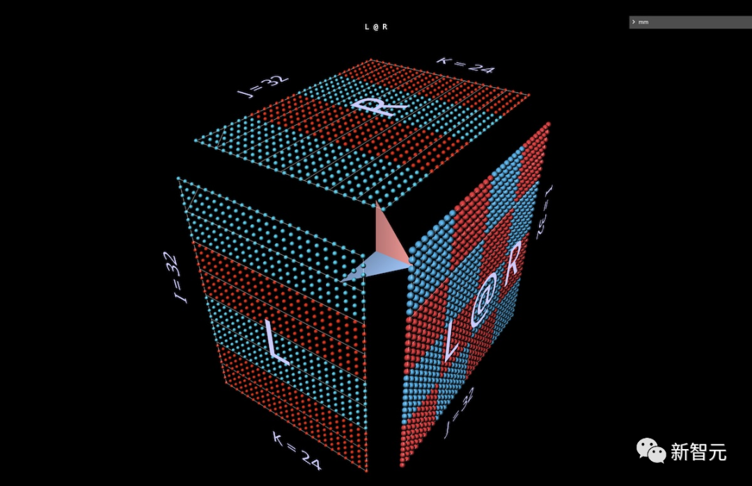
When we encase matrix multiplication around a cube in this way, the correct relationships between parameter shapes, result shapes, and shared dimensions are all established.
Now, the computation has geometric meaning:
Each position i, j in the result matrix anchors a vector running along the depth dimension k within the cube, where the horizontal plane extending from the i-th row of L intersects with the vertical plane extending from the j-th column of R. Along this vector, the (i, k) (k, j) element pairs from the two parameters meet and multiply, and the resulting product is summed along k and stored in the position i, j of the result.
This is the intuitive meaning of matrix multiplication:
– Summing along the third orthogonal dimension to derive the result matrix
To determine direction, the ‘mm’ tool displays an arrow pointing to the result matrix within the cube, with blue indicators coming from the left parameter and red indicators coming from the right parameter.
The tool also displays white guide lines to indicate the row axes of each matrix, although these guide lines are quite faint in this screenshot.
For direction, the tool shows an arrow pointing to the result matrix inside the multi-dimensional dataset, with blue leaves coming from the left parameter and red leaves coming from the right parameter. The tool also displays white guides to indicate the row axes of each matrix, although they are quite faint in this screenshot.
Of course, layout constraints are straightforward:
– The left parameter and the right parameter must be adjacent along their shared (left width/right height) dimension, which is the depth (k) dimension of matrix multiplication
This geometric figure provides us with a solid foundation to visualize all standard matrix multiplication decompositions and serves as an intuitive basis for exploring the non-trivial complex combinations of matrix multiplication.
Next, we will see the real matrix world.
Standard matrix multiplication decomposition actions
Before delving into more complex examples, the Pytorch team will introduce some intuition builders to understand how things look and feel in this visualization style.
Dot Product
First is the standard algorithm. Each result element is computed by performing a dot product on the corresponding left row and right column.
What we see in the animation is the multiplication value vector scanning inside the cube, with each vector producing a summation result at the corresponding position.
Here, the row block of L is filled with 1 (blue) or -1 (red); the column block of R is filled similarly. k is 24 here, so the blue value of the result matrix (L @ R) is 24, and the red value is -24.
Matrix-Vector Product
The matmul decomposed into a matrix-vector product looks like a vertical plane (the product of the left parameter and each column of the right parameter), which, as it sweeps horizontally through the inside of the cube, draws the columns onto the result.

Even in simple examples, observing the intermediate values of the decomposition can be very interesting.
For instance, when using randomly initialized parameters, note the prominent vertical patterns in the intermediate matrix-vector product. This reflects that each intermediate value is a scaled copy of the columns of the left parameter:
Vector-Matrix Product
The matrix multiplication decomposed into a vector-matrix product looks like a horizontal plane drawing the rows onto the result as it sweeps through the inside of the cube:
When switching to randomly initialized parameters, we see similar patterns to the matrix-vector product, but this time the pattern is horizontal, as each intermediate vector-matrix product is a scaled copy of the rows of the right parameter.
When considering how matrix multiplication expresses the rank and structure of its parameters, it is worth imagining the case where both patterns appear simultaneously in the computation:
Here is another intuition builder using vector-matrix products, showing how the identity matrix acts as a mirror, setting its parameters and results at a 45-degree angle:
Sum of Outer Products
The third plane decomposition occurs along the k-axis, calculating the outer product through vector dot products to yield the matrix multiplication result.
Here, we see the outer product plane sweeping through the cube “from back to front”, accumulating into the result:

Using randomly initialized matrices for this decomposition, we can see that with each rank-1 outer product added, not only are values accumulated in the result, but also the ranks.
Among other things, this also helps us understand why “low-rank factorization”, i.e., approximating a matrix through constructing matrix multiplications with very small deep dimension parameters, works best when the matrix being approximated is low-rank.
LoRA will be introduced later:
Expressions
How can we extend this visualization method to composite matrix multiplications?
So far, examples have visualized a single matrix L and R of the form L @ R, but what if L and/or R are matrices themselves, and so forth?
It turns out we can extend this method quite well to composite expressions.
The key rule is simple: sub-expressions (sub) matrix multiplications are another cube, subject to the same layout constraints as the parent expression, with the result face of the sub-expression simultaneously being the corresponding parameter face of the parent expression, just like covalent bonds share electrons.
Within these constraints, we can freely arrange the faces of sub-matmuls.
Here, the researchers used the tool’s default scheme, which alternates between generating convex and concave faces of cubes, a layout that is very effective in practice, maximizing space and reducing occlusion.
In this section, Pytorch will visualize some key components in ML models, to master the visual idioms and understand what intuitive feelings even simple examples can bring us.
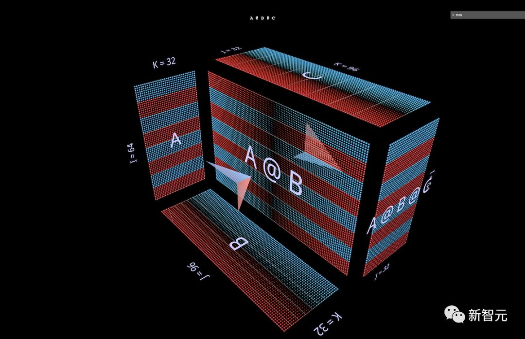
Left Associative Expressions
First, let’s look at two expressions of the form (A @ B) @ C, each having its own unique shape and characteristics.
First, we will endow (A @ B) @ C with the characteristic shape of FFN, where the “hidden dimension” is wider than the “input” or “output” dimensions. (In this case, this means B’s width is greater than A or C’s width).
Similar to a single matmul example, floating arrows point to the result matrix, with blue coming from the left parameter and red coming from the right parameter:
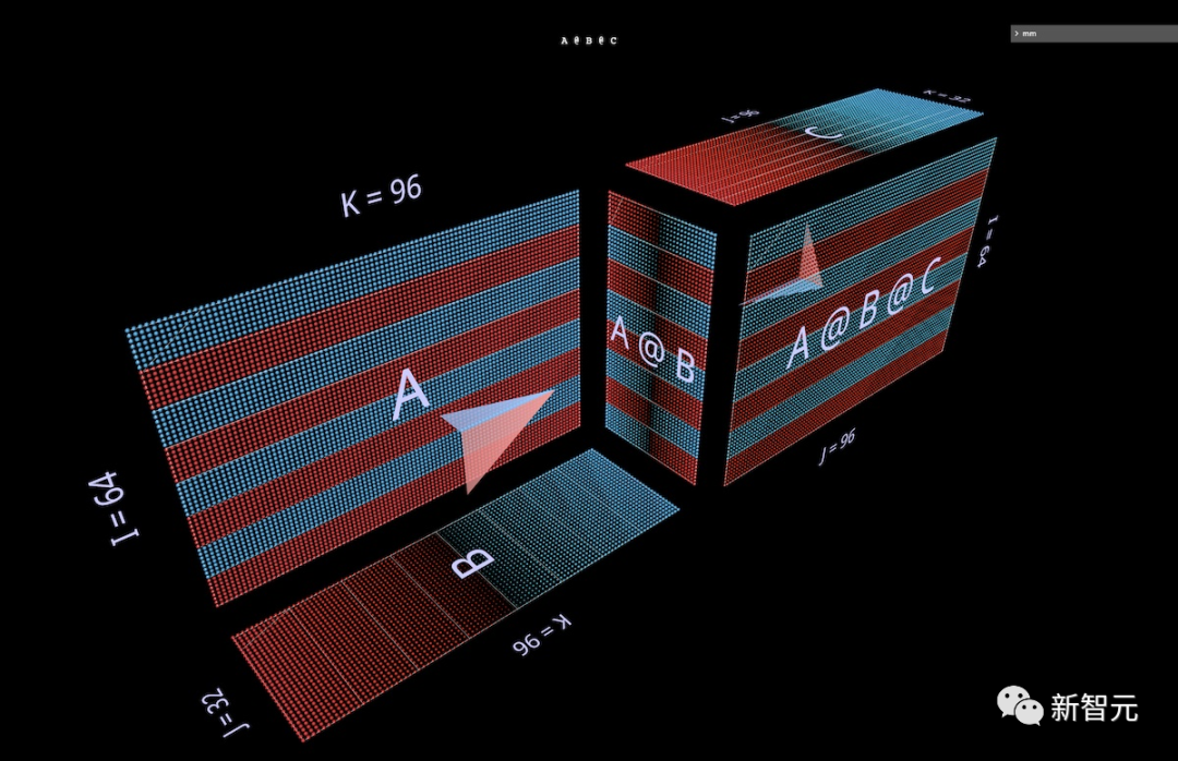
Next, we will visualize (A @ B) @ C, where B’s width is narrower than A or C, resulting in a bottleneck or “autoencoder” shape:
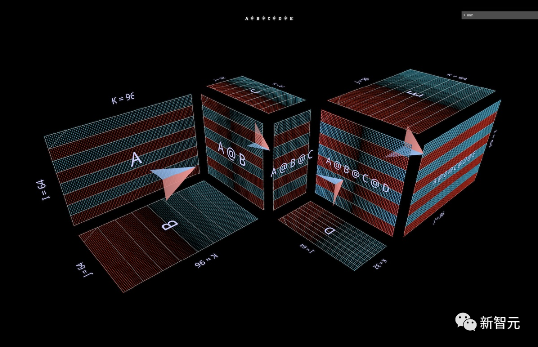
This pattern of alternating convex and concave shapes can be extended to chains of arbitrary length: for example, this multi-layer bottleneck:
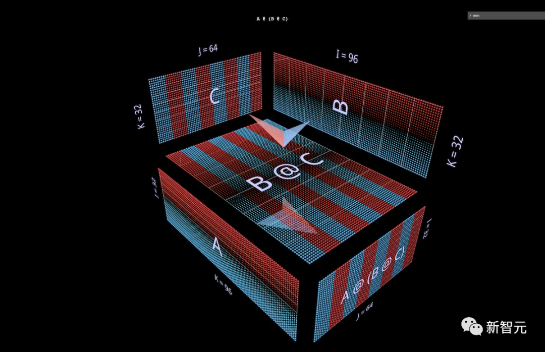
Right Associative Expressions
Next, we will visualize a right associative expression A @ (B @ C).
Sometimes, we see MLP adopt a right associative manner, where the input layer is on the right, and the weight layers go from right to left.
Using the matrix from the double-layer FFN example above—after appropriate transposition—it looks like this, where C now plays the role of input, B is the first layer, and A is the second layer:
Binary Expressions
For the visualization tool to function beyond simple teaching examples, it must maintain readability as expressions become increasingly complex.
In real-world use cases, binary expressions are a key structural component, where both sides have sub-expressions.
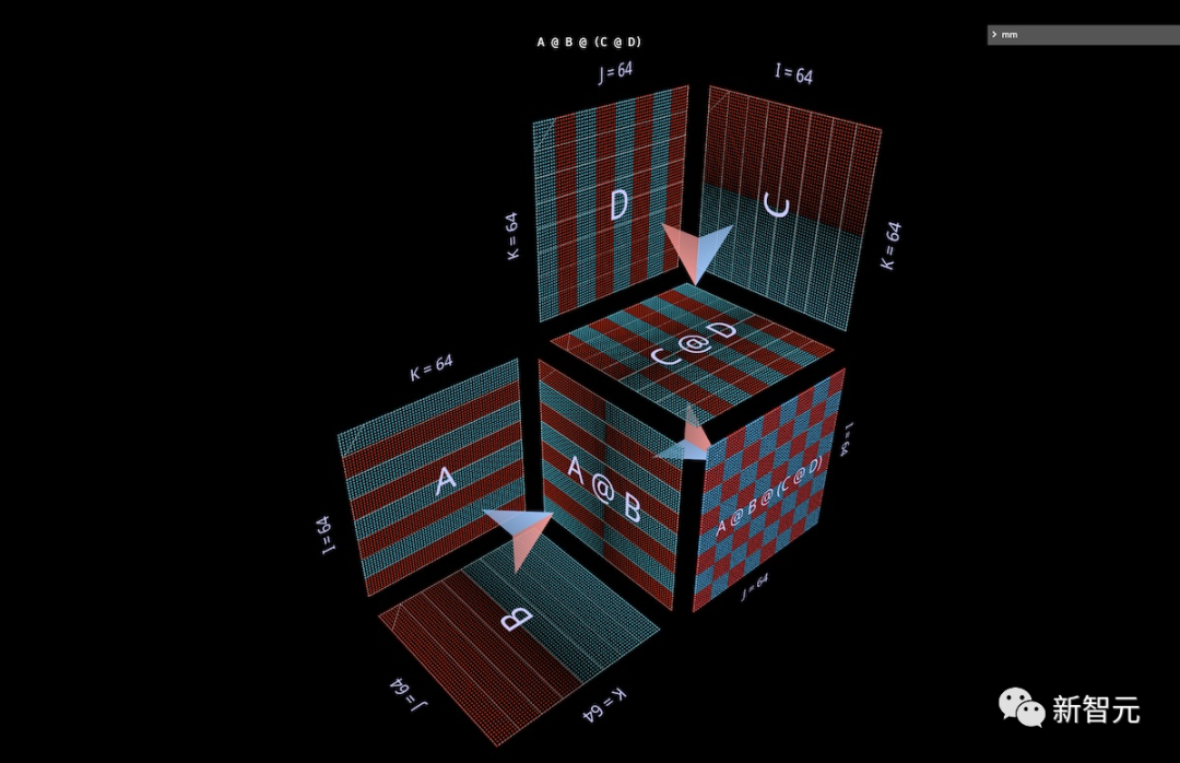
Here, we will visualize the simplest expression shape, (A @ B) @ (C @ D):
Segmentation and Parallelism
Next, we can understand how this visualization style makes the parallel reasoning of composite expressions very intuitive through two quick examples.
In the first example, we apply the standard “data parallel” segmentation to the aforementioned left associative multi-layer bottleneck example.
Segmenting along i, we segment the left initial parameters (batch) and all intermediate results (activations), but do not segment the subsequent parameters (weights).
Through the geometric figure, we can clearly see which participants in the expression are segmented and which remain intact:
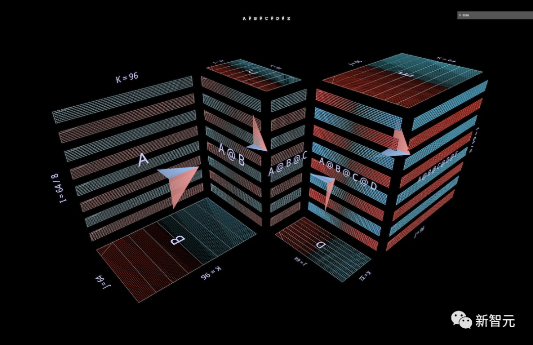
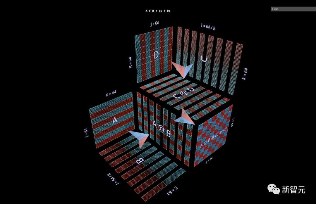
The second example demonstrates how to parallelize binary expressions by segmenting the left sub-expression along its j-axis, the right sub-expression along its i-axis, and the parent expression along its k-axis:
Attention Head Internals
Let’s look at a GPT2 attention head—specifically the “gpt2” (small) configuration from NanoGPT (layers=12, heads=12, embedding=768) at layer 5, using OpenAI weights via HuggingFace.
The input activation comes from the forward pass of 256 token training samples from OpenWebText.
The researchers chose it mainly because it computes a fairly common attention pattern and is located in the middle of the model, where activations have become structured and show some interesting textures.
Structure
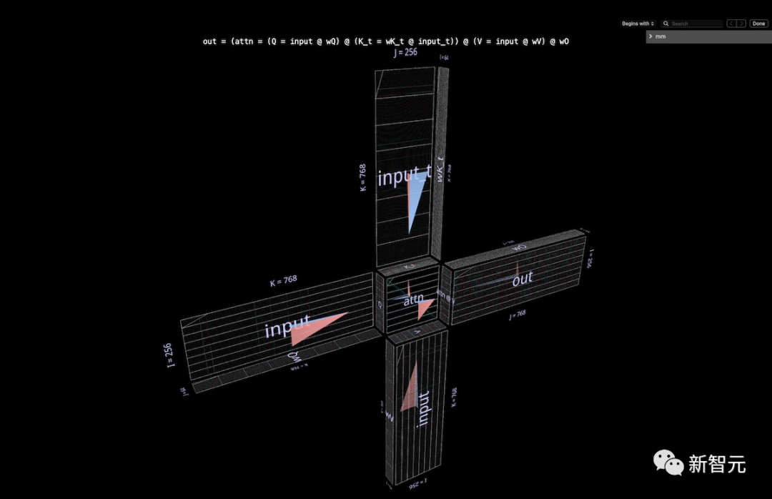
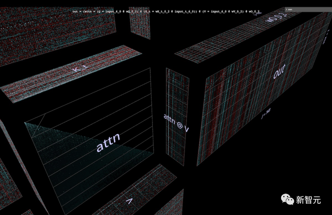
The entire attention head is visualized as a single composite expression, starting with the input and ending with the output projection. (Note: To maintain self-containment, the researchers output project each head as described in Megatron-LM).
The computation includes six matrices:
Q = input @ wQ // 1K_t = wK_t @ input_t // 2V = input @ wV // 3attn = sdpa(Q @ K_t) // 4head_out = attn @ V // 5out = head_out @ wO // 6The thumbnail description of what we are looking at:
The arrow leaves are matrix multiplications 1, 2, 3, and 6: the previous group is the inner projections from input to Q, K, and V; the latter group is the outer projection from attn @ V back to the embedding dimension.
In the center is the double matrix multiplication, which first computes the attention scores (the convex cube behind) and then uses them to generate output tokens from the value vector (the concave cube in front). Causality means the attention scores form a lower triangular matrix.
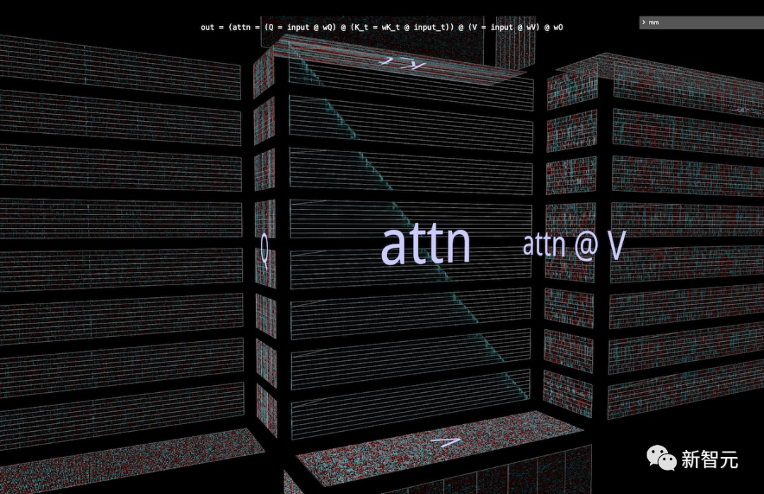
Calculations and Values
This is an animation of calculating attention. Specifically:
sdpa(input @ wQ @ K_t) @ V @ wO(i.e., the matrix 1, 4, 5, and 6 above, where K_t and V are pre-computed) the calculation process is a fused vector-matrix multiplication chain: each item in the sequence is completed in one step, covering the entire process from input to attention to output.
Differences in Heads
Before moving on to the next step, here is another demonstration that gives us a simple understanding of how the model works in detail.
This is another attention head of GPT2.
Its behavior is drastically different from the 4th head of layer 5 above, as expected, because it is located in a very different part of the model.
This head is located in the first layer: layer 0, head 2:
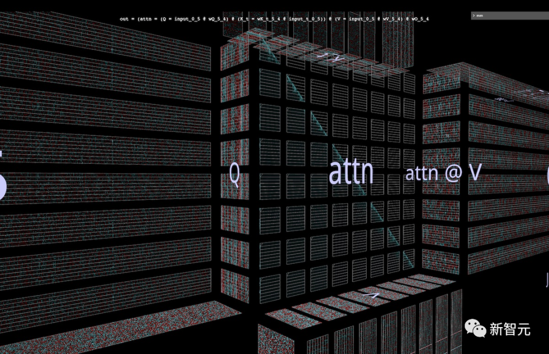
Parallel Attention
We visualize 4 of the 6 matrices in the attention head as a fused vector-matrix multiplication chain.
It is a chain that fuses vector-matrix products, confirming the geometric intuition that the entire left associative chain from input to output along the shared i-axis is layered and can be parallelized.
For example, segmenting along i:
Double partitioning:
LoRA
The recent LoRA paper describes an efficient fine-tuning technique based on the idea that the weight increments introduced during fine-tuning are low-rank.
According to the paper, this allows us to indirectly train some dense layers in neural networks while keeping the pre-trained weights frozen by optimizing the low-rank factorization matrices that change during adaptation.
Basic Idea
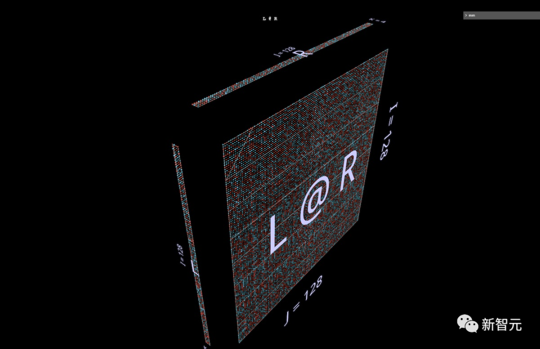
In short, the key step is to train the factor of the weight matrix rather than the matrix itself: replacing the I x J weight tensor with the matmul of an I x K tensor and a K x J tensor, keeping K as some small number.
If K is small enough, the size savings will be substantial, but at the cost that reducing K will lower the rank that the product can express.
Below is a random left 128 x 4 and right 4 x 128 parameter matmul, i.e., a rank-4 factorization of a 128 x 128 matrix, which quickly illustrates the size savings and structural impact on the result. Note the vertical and horizontal patterns of L @ R:
Download 1: OpenCV-Contrib Extension Module Chinese Tutorial
Reply to "Beginner's Guide to Vision" public account backstage: Extension Module Chinese Tutorial, to download the first OpenCV extension module tutorial in Chinese available online, covering installation of extension modules, SFM algorithms, stereo vision, object tracking, biological vision, super-resolution processing, and more than twenty chapters.
Download 2: Python Vision Practical Project 52 Lectures
Reply to "Beginner's Guide to Vision" public account backstage: Python Vision Practical Project, to download 31 practical vision projects including image segmentation, mask detection, lane line detection, vehicle counting, eyeliner addition, license plate recognition, character recognition, emotion detection, text content extraction, facial recognition, etc., to assist in quickly learning computer vision.
Download 3: OpenCV Practical Project 20 Lectures
Reply to "Beginner's Guide to Vision" public account backstage: OpenCV Practical Project 20 Lectures, to download 20 practical projects based on OpenCV, achieving advanced learning of OpenCV.

Group Chat

Welcome to join the public account reader group to exchange with peers. Currently, there are WeChat groups for SLAM, 3D vision, sensors, autonomous driving, computational photography, detection, segmentation, recognition, medical imaging, GAN, algorithm competitions, etc. (will gradually be subdivided in the future), please scan the WeChat ID below to join the group, and note: "Nickname + School/Company + Research Direction", for example: "Zhang San + Shanghai Jiao Tong University + Vision SLAM". Please follow the format for notes, otherwise, you will not be approved. After successful addition, you will be invited into the relevant WeChat group based on research direction. Please do not send advertisements in the group, otherwise, you will be removed from the group, thank you for your understanding~