Mastering the Powerful Algorithm Model: XGBoost

Core Points:Complete Summary of XGBoost Core Issues!

Hello, I am Cos Dazhuang!

Today I will share content about XGBoost~

XGBoost is very important, especially excelling in classification, regression, and ranking problems. Its practical applications include financial risk control, medical diagnosis, industrial manufacturing, and advertising click-through rate prediction. With its efficient performance and robustness, XGBoost has become the preferred algorithm in many data science competitions and real-world projects, greatly improving model accuracy and reducing overfitting risks.

Indeed, common issues are frequently encountered by everyone. Recently, some students provided feedback that they have encountered some of the issues shared in previous articles, and they found them particularly useful.

Today, I have summarized 6 issues related to XGBoost. If you have any questions, feel free to message me!

• Data Preparation Issues
• Parameter Tuning Issues
• Preventing Overfitting and Underfitting Issues
• Feature Engineering Issues
• Understanding Model Output Issues
• Tuning Strategy Issues

This is the 8th issue we answer for our readers: Mastering the Powerful Algorithm – XGBoost!!

As usual:If you think recent articles are good, please like and share them so more friends can see them.

Alright, let’s continue with the main title categorization and specific questions without further ado, let’s take a look~

If you have any questions, feel free to message me! No limits on XGBoost!

Data Preparation Issues

Reader Question: Hello Dazhuang! Recently, while processing data, I found some non-numeric features in the data. How should I handle them to use in XGBoost? Are there any tips for this?

Dazhuang’s Answer: Hello, generally speaking, handling non-numeric features in XGBoost usually requires feature engineering, as XGBoost is a tree-based algorithm that can only handle numeric features.

Here are some common tips you can look at:

1. Label Encoding

Map non-numeric features to integers. Assign a unique integer value for each category. This can be done using scikit-learn’s LabelEncoder.

from sklearn.preprocessing import LabelEncoder

label_encoder = LabelEncoder()
data['categorical_feature'] = label_encoder.fit_transform(data['categorical_feature'])

2. One-Hot Encoding

Convert non-numeric features into binary format to indicate the presence of each category. This can be achieved using pandas’ get_dummies function.

data = pd.get_dummies(data, columns=['categorical_feature'])

3. Target Encoding

Replace category labels with statistics of the target variable (e.g., mean). This helps retain relationships between categories and is particularly useful for high cardinality categories.

target_mean = data.groupby('categorical_feature')['target'].mean()
data['categorical_feature_encoded'] = data['categorical_feature'].map(target_mean)

4. Frequency Encoding

Use the occurrence frequency of each category to replace category labels. This also helps retain the relative relationships between categories.

freq_encoding = data['categorical_feature'].value_counts(normalize=True)
data['categorical_feature_encoded'] = data['categorical_feature'].map(freq_encoding)

5. Embedding Encoding

For high cardinality non-numeric features, you can use embedding layers to learn representations. This is more common in neural networks and can be implemented using PyTorch.

import torch
import torch.nn as nn

class EmbeddingNet(nn.Module):
    def __init__(self, num_embeddings, embedding_dim):
        super(EmbeddingNet, self).__init__()
        self.embedding = nn.Embedding(num_embeddings, embedding_dim)

    def forward(self, x):
        return self.embedding(x)

# Example usage
embedding_model = EmbeddingNet(num_embeddings=len(data['categorical_feature'].unique()), embedding_dim=10)
embedded_data = torch.tensor(data['categorical_feature'].values, dtype=torch.long)
result = embedding_model(embedded_data)

6. Custom Transformations

Based on business logic, other custom methods can be used to convert non-numeric features into numeric features.

In practical applications, you can choose appropriate methods based on the nature of the data and the requirements of the problem. It is also recommended to use cross-validation and other techniques to evaluate the impact of different encoding methods on model performance.

In specific practice, especially when using models like XGBoost, you need to weigh and choose based on the specific problems and characteristics of the dataset.

If you have any questions, feel free to message me~

Parameter Tuning Issues

Reader Question: I want to ask a question, generally speaking, what is the subsample ratio and column sample ratio, and how should I adjust these parameters?

Dazhuang’s Answer: Hello, in XGBoost, the subsample ratio and column sample ratio are two important hyperparameters used to control the sampling ratio of training data and features for each tree.

Adjusting these two parameters can significantly impact model performance.

1. Subsample Ratio (subsample):

• Definition: It indicates the proportion of training samples for each tree. The value ranges from 0 to 1.
• Function: Controls the sampling ratio of training data for each tree, which can prevent overfitting.
• Adjustment Method: If the model is overfitting, you can reduce this value; if the model is underfitting, you can moderately increase it.

params = {
    'subsample': 0.8  # For example, set the subsample ratio to 0.8
}

2. Column Sample Ratio (colsample_bytree):

• Definition: It indicates the feature sampling ratio for each tree. The value ranges from 0 to 1.
• Function: Controls the sampling ratio of features for each tree, which can increase model diversity.
• Adjustment Method: If the feature dimension is high, you can moderately reduce this value; if the model is overfitting on features, you can increase this value.

params = {
    'colsample_bytree': 0.9  # For example, set the column sample ratio to 0.9
}

3. Other Related Parameters:

• XGBoost also has other sampling-related parameters, such as colsample_bylevel (column sample ratio for each level) and colsample_bynode (column sample ratio for each node). These parameters can be adjusted based on actual circumstances.

params = {
    'colsample_bylevel': 0.8,  # For example, set the column sample ratio for each level to 0.8
    'colsample_bynode': 0.7   # For example, set the column sample ratio for each node to 0.7
}

4. Tuning Process:

• Use cross-validation and other methods to try different combinations of subsample ratios and column sample ratios.
• You can use Grid Search or Random Search methods to find the optimal hyperparameter combinations.

5. A Complete Example:

• Here is a simple example code for training and tuning an XGBoost model:

import xgboost as xgb
from sklearn.datasets import load_boston
from sklearn.model_selection import train_test_split
from sklearn.metrics import mean_squared_error
import matplotlib.pyplot as plt

# Load dataset
data = load_boston()
X_train, X_test, y_train, y_test = train_test_split(data.data, data.target, test_size=0.2, random_state=42)

# Define parameters
params = {
    'objective': 'reg:squarederror',
    'subsample': 0.8,
    'colsample_bytree': 0.9,
    'max_depth': 3,
    'learning_rate': 0.1,
    'n_estimators': 100
}

# Create model
model = xgb.XGBRegressor(**params)

# Train model
model.fit(X_train, y_train)

# Predict
y_pred = model.predict(X_test)

# Evaluate model
mse = mean_squared_error(y_test, y_pred)
print(f'Mean Squared Error: {mse}')

# Plot feature importance
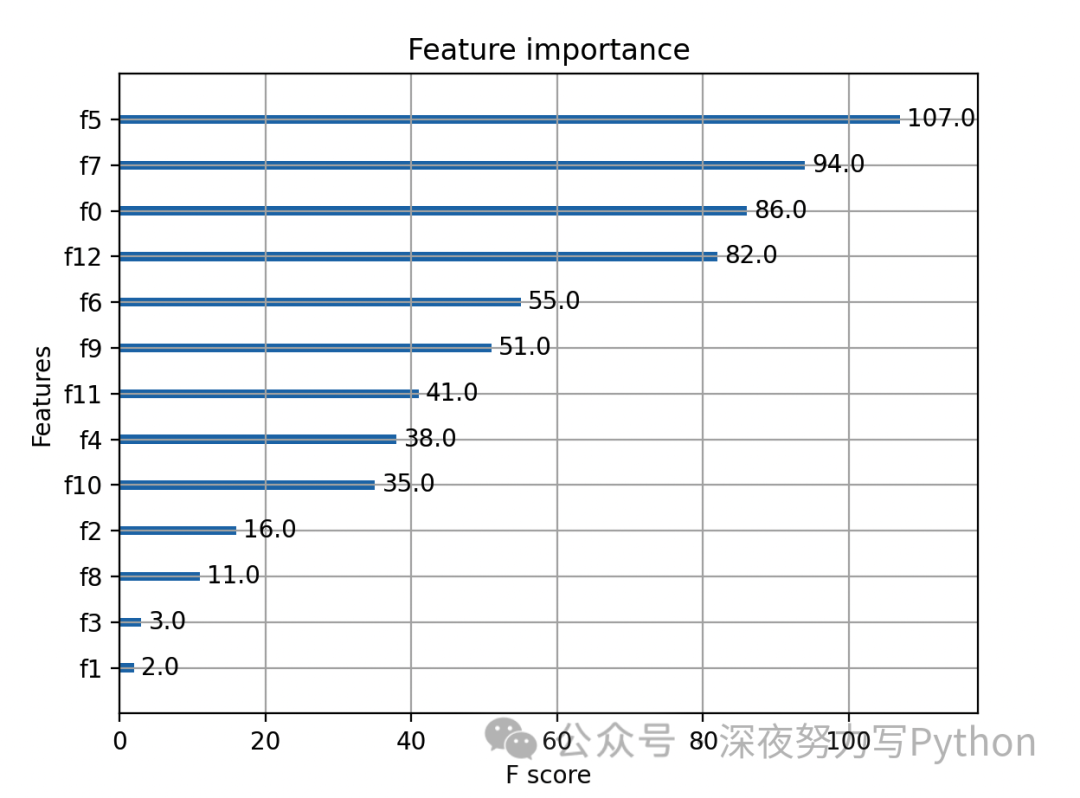
xgb.plot_importance(model)
plt.show()

In the above code, subsample and colsample_bytree set the subsample ratio and column sample ratio, and other parameters can be adjusted based on specific circumstances. The feature importance plot can be used for further analysis of the model’s performance.

Preventing Overfitting and Underfitting Issues

Reader Question: I saw content on Early Stopping, but I’m still not clear. Is it used to prevent overfitting? How is it used in XGBoost?

Dazhuang’s Answer: Hello, yes, it is used to prevent overfitting. Early Stopping is a technique used to prevent overfitting by monitoring the performance metrics of the model during training and stopping training early when the model performance stops improving, thus preventing the model from overfitting on the training set and improving its generalization ability.

In XGBoost, the main goal of Early Stopping is to monitor the performance of the validation set and stop training when performance no longer improves.

Here are the general steps on how to use Early Stopping in XGBoost:

1. Prepare the Dataset: Split the dataset into training and validation sets, usually using cross-validation.

2. Define the Model: Use XGBoost’s Python interface (xgboost package) to define a basic model, setting basic parameters like learning rate, max depth, etc.

3. Configure Early Stopping Parameters: Set parameters related to Early Stopping, mainly including early_stopping_rounds and eval_metric. early_stopping_rounds indicates how many rounds of performance on the validation set must not improve before stopping training. eval_metric is the metric used to evaluate model performance; for example, you can choose ‘logloss’ as the evaluation metric.

4. Train the Model: Fit the model using the training dataset while also passing in the validation dataset to monitor the model’s performance on the validation set.

5. Apply Early Stopping: During training, when the performance on the validation set does not improve for the specified number of rounds, training will stop early. This is achieved by setting the early_stopping_rounds parameter.

Finally, here is a code example:

import xgboost as xgb
from sklearn.model_selection import train_test_split
from sklearn.datasets import load_boston
from sklearn.metrics import mean_squared_error
import matplotlib.pyplot as plt

# Load example dataset
boston = load_boston()
X, y = boston.data, boston.target

# Split training and validation sets
X_train, X_valid, y_train, y_valid = train_test_split(X, y, test_size=0.2, random_state=42)

# Convert data to DMatrix format
dtrain = xgb.DMatrix(X_train, label=y_train)
dvalid = xgb.DMatrix(X_valid, label=y_valid)

# Define model parameters
params = {
    'objective': 'reg:squarederror',
    'eval_metric': 'rmse',
    'eta': 0.1,
    'max_depth': 5,
    'subsample': 0.8,
    'colsample_bytree': 0.8
}

# Define Early Stopping parameter
early_stopping_rounds = 10

# Train model and apply Early Stopping
model = xgb.train(params, dtrain, num_boost_round=1000, evals=[(dtrain, 'train'), (dvalid, 'valid')],
                  early_stopping_rounds=early_stopping_rounds, verbose_eval=True)

# Evaluate model performance on test set
y_pred = model.predict(dvalid, ntree_limit=model.best_ntree_limit)
mse = mean_squared_error(y_valid, y_pred)
print(f"Mean Squared Error on Validation Set: {mse}")

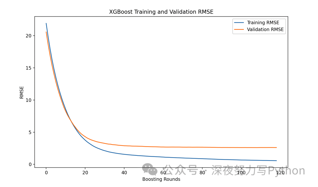
# Plot performance over training rounds
xgb.plot_metric(model)
plt.show()

In the above example, the model will monitor performance on the validation set, and if performance does not improve for 10 consecutive rounds (which can be adjusted based on actual conditions), training will stop. Finally, the code visualizes the performance over training rounds.

Feature Engineering Issues

Reader Question: Dazhuang, I just started learning and want to ask a question. What are cross features? Do creating new features help improve model performance?

Dazhuang’s Answer: Hello, in your experiments, cross features are as follows. They usually refer to introducing new features by combining different features to capture the interaction relationships between features. This feature engineering technique helps improve model performance because it can better capture non-linear relationships and interaction effects in the data. By introducing cross features, the model can better adapt to the complexity of the data, thereby improving its predictive capability for the target.

This is the capability provided by cross features. Therefore, it is very important, and I have summarized the importance in a few points:

1. Capturing Non-Linear Relationships: By introducing cross features, the model can better capture non-linear relationships between different features, thus enhancing the model’s expressive power.

2. Increasing Information: Cross features can introduce new information, helping the model better understand hidden patterns and rules in the data.

3. Handling Interaction Effects Between Features: Features in data are often not isolated; they have complex interaction effects. By introducing cross features, the model can better capture these interaction effects, enhancing the model’s generalization ability.

4. Increasing Model Complexity: The introduction of cross features increases the complexity of the model, allowing it to better adapt to complex data structures and improve its predictive ability for unseen data.

Below, I wrote an example. Suppose we have two features x1 and x2, by introducing the cross feature x1 * x2, we can capture the multiplicative relationship between x1 and x2. You can take a look at this example~

import numpy as np
import pandas as pd
from sklearn.model_selection import train_test_split
from sklearn.preprocessing import LabelEncoder
import xgboost as xgb
from sklearn.metrics import accuracy_score

# Create example data
np.random.seed(42)
X = pd.DataFrame({'x1': np.random.rand(100), 'x2': np.random.rand(100)})
y = (3*X['x1'] + 2*X['x2'] + 0.5*X['x1']*X['x2'] + 0.1*np.random.randn(100) > 0).astype(int)

# Use LabelEncoder to convert y to integer labels starting from 0
y_encoded = label_encoder.fit_transform(y)

# Split training and testing sets
X_train, X_test, y_train, y_test = train_test_split(X, y_encoded, test_size=0.2, random_state=42, stratify=y_encoded)

# Build XGBoost model
model = xgb.XGBClassifier()
model.fit(X_train, y_train)

# Predict
y_pred = model.predict(X_test)

# Calculate accuracy
accuracy = accuracy_score(y_test, y_pred)
print(f"Accuracy: {accuracy}")

In this example, by introducing the cross feature x1 * x2, we increased the model’s fitting ability and improved classification accuracy. In practice, the selection and creation of cross features need to be based on specific problems and characteristics of the data, and domain knowledge or feature importance methods can guide the feature engineering process.

If you have questions, feel free to message me~

Understanding Model Output Issues

Reader Question: What is the structure of each tree in the model and how to understand the decision path?

Dazhuang’s Answer: Here’s the thing. Each tree’s structure and decision path consist of multiple decision nodes and leaf nodes. XGBoost uses a gradient boosting algorithm, iteratively training a series of decision trees and combining them to form a powerful ensemble model.

1. Decision Nodes (Split Node): At each node of the tree, there is a decision condition based on a threshold of an input feature. Decision nodes split the dataset into two subsets, based on whether the feature value meets the condition.

Where is the chosen feature, and is the threshold for that feature.

2. Leaf Nodes (Leaf Node): At the end of the tree, leaf nodes contain a prediction value. When an input sample reaches a certain leaf node through the decision path of the tree, the prediction value of that leaf node will be used for the final model prediction.

3. Tree Structure: Each tree in XGBoost is depth-limited, and limiting the depth of the tree can effectively prevent overfitting. The structure of the tree consists of a hierarchy of decision nodes and leaf nodes, forming a binary tree structure. The depth of the tree is usually controlled by hyperparameters.

4. Decision Path: Each sample moves through a decision path on the tree, starting from the root node and gradually moving down according to the decision conditions at each node until reaching a leaf node. The decision path is a series of decision nodes that the sample passes through, and the decision conditions of these nodes constitute the decision process of the sample.

5. Understanding the Decision Path: By analyzing the structure of each tree and the decision path, we can understand how the model combines and weights the input features. Important features will appear at the upper nodes of the tree, while less important features may appear at deeper nodes. The decision path also reflects how the model combines different features to make the final prediction.

Finally, we can use the xgboost library to implement XGBoost with PyTorch. To understand the structure of each tree and the decision path, you can use the plot_tree function to visualize a single tree.

import numpy as np
import xgboost as xgb
import matplotlib.pyplot as plt

# Create a fictitious dataset
np.random.seed(42)
X_train = np.random.rand(100, 5)  # Assume 100 samples, each with 5 features
y_train = np.random.rand(100)     # Corresponding target variable

# Create XGBoost model
model = xgb.XGBRegressor()

# Train model
model.fit(X_train, y_train)

# Visualize the first tree
plt.figure(figsize=(20, 10))
xgb.plot_tree(model, num_trees=0, rankdir='LR')
plt.show()

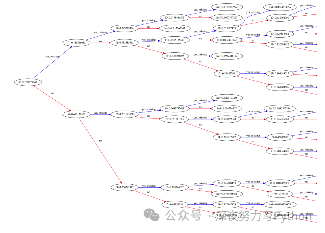
Through this visualization, you can see the structure of the tree, the features and thresholds at each node, and the output values at the leaf nodes, which helps better understand the decision path of the model.

In summary, understanding the structure of each tree and the decision path in the XGBoost model helps us gain insights into how the model makes predictions, thus facilitating model interpretation and tuning.

Tuning Strategy Issues

Reader Question: What is the difference between grid search and random search? Which method should I choose when tuning parameters?

Dazhuang’s Answer: Okay, first you need to know that grid search (Grid Search) and random search (Random Search) are commonly used tuning methods, and their main difference lies in the way they search the parameter space.

Below, I will elaborate on the differences between these two methods and the considerations for choosing a method during tuning.

1. Grid Search

• Principle: Grid search is an exhaustive search method that searches through all possible combinations of predefined parameters in the parameter space. By specifying different parameter combinations, grid search traverses all possible combinations to find the optimal parameters.
• Advantages: Simple and intuitive, with a higher possibility of finding the global optimal solution.
• Disadvantages: High computational overhead, especially when the parameter space is large, requiring a lot of time and computational resources.

from sklearn.model_selection import GridSearchCV

# Define parameter grid
param_grid = {
    'learning_rate': [0.1, 0.01, 0.001],
    'max_depth': [3, 5, 7],
    'n_estimators': [50, 100, 200]
}

# Create GridSearchCV object
grid_search = GridSearchCV(estimator=xgboost_model, param_grid=param_grid, cv=5)
grid_search.fit(X_train, y_train)

2. Random Search

• Principle: Random search samples a set of parameters randomly from the parameter space and then evaluates model performance. This process is repeated multiple times until the specified number of searches or time is reached. Compared to grid search, random search emphasizes randomness and explores the parameter space more broadly through random sampling.
• Advantages: Relatively low computational overhead, capable of finding better parameter combinations in a shorter time.
• Disadvantages: It may not find the global optimal solution, but it can find a good local optimal solution in a shorter time.

from sklearn.model_selection import RandomizedSearchCV

# Define parameter distribution
param_dist = {
    'learning_rate': [0.1, 0.01, 0.001],
    'max_depth': [3, 5, 7],
    'n_estimators': [50, 100, 200]
}

# Create RandomizedSearchCV object
random_search = RandomizedSearchCV(estimator=xgboost_model, param_distributions=param_dist, n_iter=10, cv=5)
random_search.fit(X_train, y_train)

3. Considerations for Choosing a Method

• Computational Resources: If computational resources are abundant, you can consider using grid search to ensure exhaustive search of the parameter space. If resources are limited, random search may be a better option.
• Parameter Space: If the parameter space is small, grid search may be a good choice. If the parameter space is large, random search has an advantage.
• Time Efficiency: If time is limited, random search may be more suitable as it can find better parameter combinations in a relatively short time.

In general, both grid search and random search are effective tuning methods, and the choice depends on the specific situation. In practice, you can also combine these two methods, first using random search to narrow down the search space, and then using grid search for finer tuning in the narrowed space.

FAQ Summary

Mastering the Powerful Algorithm Model, Regression!

Mastering the Powerful Algorithm Model, Decision Trees!

Mastering the Powerful Algorithm Model, Clustering!

Mastering the Powerful Algorithm Model, SVM!

Mastering the Powerful Algorithm Model, KNN!

Mastering the Powerful Algorithm Model, Random Forests!

Mastering the Powerful Algorithm Model, Naive Bayes!

Finally

Today, I summarized FAQs about XGBoost. If you have questions, feel free to message me, and I will definitely reply when I see it and have time!

I have prepared a PDF version of《Machine Learning Interview Book》, light and dark versions!

16 major sections, 124 questions summarized!

How to get it? Just message me on WeChat! (Note “Interview Questions”)

In addition, we recently released《100 Powerful Machine Learning Algorithm Models》!!

Many beginners face the pain point of needing complete cases to boost their learning journey! Now, 1200 people have already joined!

For details, click here:100 Powerful Algorithm Models!!

If you like this article, pleasesave, like, and share!!

Follow this account to bring more algorithm practical examples and improve work and study efficiency!

Recommended Reading: Complete Route of Machine Learning!
Summary of Regression Algorithms!
Detailed Summary of SVM Algorithms!
Detailed Explanation of 5 Distance Algorithms!
Detailed Explanation of Overfitting and Underfitting!
Complete Summary of Regularization Algorithms!
Complete Summary of Artificial Neural Networks!
27 Powerful Python Libraries!
A Comprehensive Overview of Statistics Knowledge!
Advantages and Disadvantages of Various Machine Learning Algorithms!
Explanation of 9 Core Machine Learning Algorithms!
Final Part: Comprehensive Overview of Statistics Knowledge!

Here comes! The Most Powerful Python Analysis Tools!

7 Aspects, 30 Most Powerful Datasets!!

Transparent! A Comprehensive Overview of 10 Loss Functions!!

Summary of Supervised Learning Algorithm Cases with sklearn!
Summary of Unsupervised Learning Algorithm Cases with sklearn!
Comprehensive Summary of 20 Machine Learning Algorithms in 6 Parts!!