

Since the 1940s, deep learning has developed rapidly, achieving great success and being widely used in smartphones, cars, and many other devices.
So, what are neural networks, and what can they do?
Now, let’s focus on the classic approach in computer science:
Programmers design an algorithm that generates output data for given input data.
Programmers accurately design all the logic of the function f(x):
-
y = f(x)
-
where x and y are the input and output data, respectively
However, sometimes designing f(x) may not be so easy. For example, suppose x is a facial image, and y is the name of the communicator. This task is very easy for the brain but difficult for computer algorithms!
This is where deep learning and neural networks shine.
The basic principle is: abandon the f() algorithm and try to mimic the brain.
So how does the brain perform?
The brain continually trains using several infinite pairs (x, y) samples (training sets), during which the f(x) function is automatically formed. It is not designed by anyone but is formed from an endless trial-and-error refinement mechanism.
Think of a child who looks at familiar people around them every day: billions of snapshots taken from different locations, perspectives, and lighting conditions, each recognition involves association, correction, and sharpening of the natural neural network.
Artificial neural networks are models of natural neural networks composed of neurons and synapses in the brain.
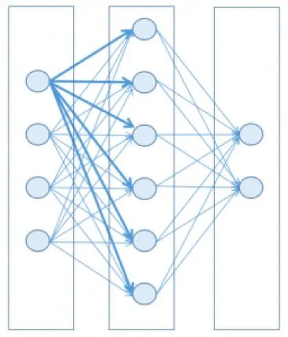
Typical neural network structure
To keep it simple and leverage today’s mathematical and computational capabilities, neural networks can be designed as a set of layers, each containing nodes (the artificial counterparts of brain neurons), where each node in a layer is connected to nodes in the next layer.
Each node has a state represented by a floating-point number, usually ranging from 0 to 1. When the state is close to its minimum value, the node is considered inactive (off), and when it is close to its maximum value, the node is considered active (on). You can think of it as a light bulb; it does not strictly rely on a binary state but is at some intermediate value within the range.
Each connection has a weight, so the active nodes in the previous layer will influence the activity of the nodes in the next layer (excitatory connections), while inactive nodes will not have any effect.
The weights of the connections can also be negative, meaning that the nodes in the previous layer (to a greater or lesser extent) influence the inactivity of the nodes in the next layer (inhibitory connections).
In simple terms, let’s assume a subset of a network where three nodes in the previous layer are connected to a node in the next layer. In short, assume the first two nodes in the previous layer are at their maximum activation value (1), while the third node is at its minimum value (0).
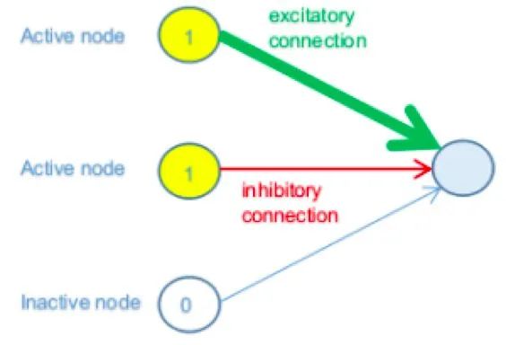
In the above image, the first two nodes in the previous layer are active (on), so they contribute to the state of the node in the next layer, while the third node is inactive (off), so it does not influence in any way (regardless of its connection weight).
The first node has a strong (thick) positive (green) connection weight, meaning it contributes significantly to activation. The second has a weak (thin) negative (red) connection weight; therefore, it helps to inhibit the connected node.
Finally, the weighted sum of all contributions from the incoming connection nodes from the previous layer is obtained.
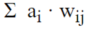
Where i is the activation state of node i, and w_ij is the connection weight between node i and node j.
So, given the weighted sum, how do we determine if the node in the next layer will be activated? Does the rule really work like “the sum is positive, then activated; the result is negative, then not activated”? It could be, but generally, it depends on which activation function and threshold you choose for that node.
Think about it. This final number can be any number in the real range, and we need to use it to set the node state within a more limited range (let’s say from 0 to 1). Then we map the first range to the second range to compress any (negative or positive) number into the range of 0 to 1.
The sigmoid function is a common activation function that performs this task.
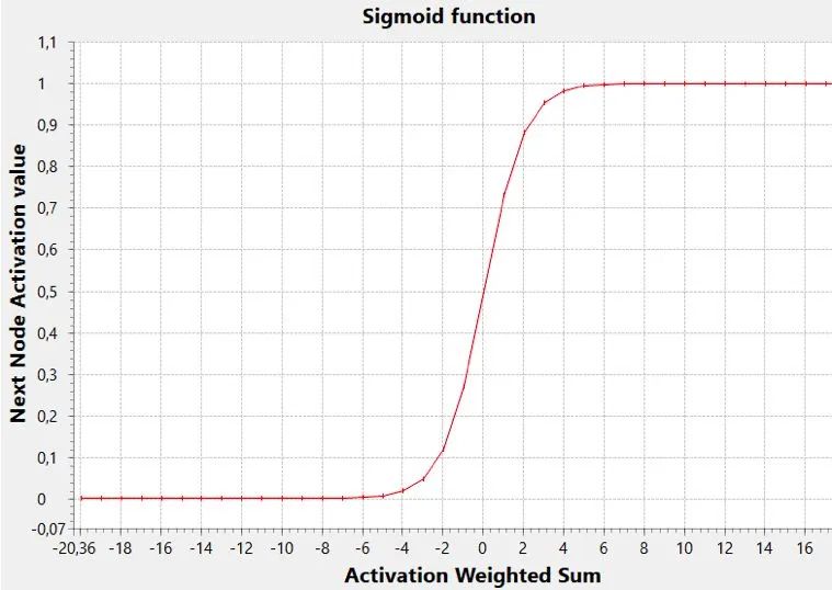
In this graph, the threshold (the x value where the y value reaches the middle of the range, i.e., 0.5) is zero, but generally, it can be any value (negative or positive, which affects the sigmoid’s left or right movement).
A low threshold allows the activation of nodes with lower weighted sums, while a high threshold will only activate based on high values of that sum.
This threshold can be implemented by considering additional virtual nodes in the previous layer, which have a constant activation value of 1. In this case, the connection weight of this virtual node can serve as the threshold, and the sum formula mentioned above can be considered to include the threshold itself.
Ultimately, the state of the network is represented by a set of values of all its weights (broadly speaking, including the threshold).
A given state or set of weight values may produce poor results or large errors, while another state may produce good results, in other words, small errors.
Therefore, moving in an N-dimensional state space can cause small or large errors. The loss function can map the weight domain to a function of error values. In n+1 space, it is hard for people to imagine such a function. However, for N = 2, it is a special case.
Training a neural network involves finding the minimum loss function. Why is it the best minimum rather than the global minimum? It is actually because this function is often non-differentiable, so it can only wander in the weight domain using some gradient descent techniques, avoiding the following situations:
-
Making too large changes, you might miss the best minimum without realizing it
-
Making too small changes, you might get stuck in a not-so-good local minimum
Not easy, right? This is the main issue with deep learning and explains why the training phase can take hours, days, or even weeks.
This is why hardware is crucial for this task, and it also explains why it is often necessary to pause, consider different methods, and reconfigure parameters to restart.
Now back to the general structure of the network, which is a stack of layers. The first layer is the input data (x), while the last layer is the output data (y).
The intermediate layers can be zero, one, or multiple. They are called hidden layers, and the term “depth” in deep learning refers to the fact that the network can have many hidden layers, potentially finding more features that relate inputs to outputs during training.
Tip: In the 1990s, you would have heard about multilayer networks instead of deep networks, but they are the same thing. It is now increasingly clear that the further the filtering layers are from the input layer (deeper), the better they can capture abstract features.
Learning process
At the beginning of the learning process, weights are randomly set, so a given input set in the first layer will transfer and generate random (calculated) output data. The actual output data is compared with the expected output data; the difference is the measure of network error (loss function).
This error is then used to adjust the connection weights that generated it, starting from the output layer and gradually moving back to the first layer.
The amount of adjustment can be small or large and is usually defined by a factor called the learning rate.
This algorithm is called backpropagation, and it became popular after the research by Rumelhart, Hinton, and Williams in 1986.
Remember this name: Geoffrey Hinton, who is known as the “godfather of deep learning” and is a tireless scientist guiding others forward. For example, he is now researching a new paradigm called Capsule Neural Networks, which sounds like another great revolution in the field!
Backpropagation aims to gradually reduce the overall error of the network by making appropriate corrections to the weights concentrated on each iteration of training. Additionally, reducing this error is challenging because there is no guarantee that weight adjustments always move in the right direction towards minimization.
In short, it’s like walking around blindfolded trying to find a minimum on an n-dimensional surface: you might find a local minimum but never know if you can find a smaller one.
If the learning rate is too low, the process may be too slow, and the network may also get stuck in a local minimum. On the other hand, a higher learning rate may cause it to skip the global minimum and make the algorithm diverge.
In fact, the problem during the training phase is that errors only accumulate!
Current Situation
Why has this field achieved such great success now?
Mainly for the following two reasons:
-
The availability of large amounts of data required for training (from smartphones, devices, IoT sensors, and the internet)
-
The computational power of modern computers can significantly shorten the training phase (it is common for the training phase to take only weeks or even days)
Want to learn more? Here are a few good books to recommend:
-
Deep Learning by Adam Gibson and Josh Patterson, O’Reilly Media.
-
Practical Convolutional Neural Networks by Mohit Sewark, Md Rezaul Karim, and Pradeep Pujari, Packt Publishing.
—Copyright Statement—
Source: Dolphin Data Science Lab, Edited by Yu Di
For academic sharing only, copyright belongs to the original author.