KNN Principles and Six Use Cases

Nearest Neighbor Algorithm

Algorithm Principles

The principle of the nearest neighbor method is to find a predefined number of training samples that are closest to the new point and predict the label from them. The number of samples can either be a user-defined constant (k-nearest neighbor learning) or can vary based on the local density of points (radius-based neighbor learning).

sklearn.neighbors

sklearn.neighbors is a module provided in the scikit-learn library for implementing neighbor-based learning methods, including both unsupervised and supervised learning. The unsupervised nearest neighbor method serves as the foundation for many other learning methods, particularly manifold learning and spectral clustering.

Distance can be any metric: the standard Euclidean distance is the most common choice. Neighbor methods are referred to as non-generalizing machine learning methods because they simply “remember” all the training data.

Comparison of Neighbor Algorithms

Brute Force Algorithm

Fast computation of nearest neighbors is an active research area in machine learning. The simplest implementation of nearest neighbor search involves calculating the distance between all pairs of points in the dataset: for N samples in D dimensions, the complexity of this method is O[D * N^2].

For small data samples, an efficient brute force nearest neighbor search can be very competitive. However, as the number of samples N increases, the brute force method quickly becomes impractical. The brute force nearest neighbor search can be specified by the keyword algorithm = 'brute', and calculations can be performed using routines available in sklearn.metrics.pairwise.

K-D Tree

To address the computational efficiency issues of the brute force method, various tree-based data structures have been invented. Overall, these structures attempt to reduce the number of distance calculations required by efficiently encoding the aggregate distance information of the samples. The basic idea is that if point A is far from point B, and point B is close to point C, then we know that point A is far from point C without explicitly calculating their distance. In this way, the computational cost of nearest neighbor search can be reduced to O[D N log(N)] or better. This is a significant improvement for large N.

The KD tree is a binary tree structure that recursively partitions the parameter space along the data axes, dividing it into nested orthogonal regions where data points are assigned. Building a KD tree is very fast: since it only partitions along the data axes, there is no need to calculate distances in D dimensions.

Ball Tree

To address the inefficiency of KD trees in high dimensions, the ball tree data structure was developed. Unlike KD trees, which partition data along Cartesian coordinate axes, the ball tree partitions data using a series of nested hyperspheres. This results in a higher construction cost for the ball tree compared to the KD tree, but the result is a data structure that is very efficient on highly structured data, even in very high dimensions.

The ball tree recursively partitions data into nodes defined by a centroid C and a radius r, so that every point in the node lies within the hypersphere defined by r and C. By using the triangle inequality, the need for distance calculations is reduced; through this setup, a single distance calculation between the test point and the centroid is sufficient to determine the lower and upper bounds of the distances to all points within the node. Due to the spherical geometric structure of ball tree nodes, it may outperform KD-tree in high dimensions, although actual performance heavily depends on the structure of the training data.

Choosing a Nearest Neighbor Algorithm

The best algorithm for a given dataset is a complex choice that depends on many factors:

• Number of samples N (i.e., n_samples) and dimensionality D (i.e., n_features).
• Brute force query time scales with O[D N]
• Ball tree query time scales with O[D log(N)]
• KD tree query time scales with D, making it difficult to characterize precisely. For small D (around less than 20), the cost is about O[D log(N)], and KD tree queries can be very efficient. For larger D, the cost increases to nearly O[DN], and due to the overhead of the tree structure, queries may be slower than brute force.
• The number of neighbors requested for the query point k.
• Brute force query time is largely unaffected by the value of k.
• Ball tree and KD tree query times slow down as k increases.

Case 1: Unsupervised Nearest Neighbors

NearestNeighbors implements unsupervised nearest neighbor learning and serves as a unified interface for three different nearest neighbor algorithms (BallTree, KDTree, and brute force based on routines in sklearn.metrics.pairwise).

The neighbor search algorithm can be controlled by the keyword algorithm, which must be one of ['auto', 'ball_tree', 'kd_tree', 'brute']. When passing the default value ‘auto’, the algorithm will attempt to determine the best method from the training data.

>>> from sklearn.neighbors import NearestNeighbors
>>> import numpy as np
>>> X = np.array([[-1, -1], [-2, -1], [-3, -2], [1, 1], [2, 1], [3, 2]])
>>> nbrs = NearestNeighbors(n_neighbors=2, algorithm='ball_tree').fit(X)
>>> distances, indices = nbrs.kneighbors(X)
>>> indices
array([[0, 1],
       [1, 0],
       [2, 1],
       [3, 4],
       [4, 3],
       [5, 4]]...)
>>> distances
array([[0.        , 1.        ],
       [0.        , 1.        ],
       [0.        , 1.41421356],
       [0.        , 1.        ],
       [0.        , 1.        ],
       [0.        , 1.41421356]])

Since the query set matches the training set, the nearest neighbor for each point is itself, with a distance of zero. Additionally, a sparse graph displaying connections between adjacent points can be efficiently generated:

>>> nbrs.kneighbors_graph(X).toarray()
array([[1., 1., 0., 0., 0., 0.],
       [1., 1., 0., 0., 0., 0.],
       [0., 1., 1., 0., 0., 0.],
       [0., 0., 0., 1., 1., 0.],
       [0., 0., 0., 1., 1., 0.],
       [0., 0., 0., 0., 1., 1.]])

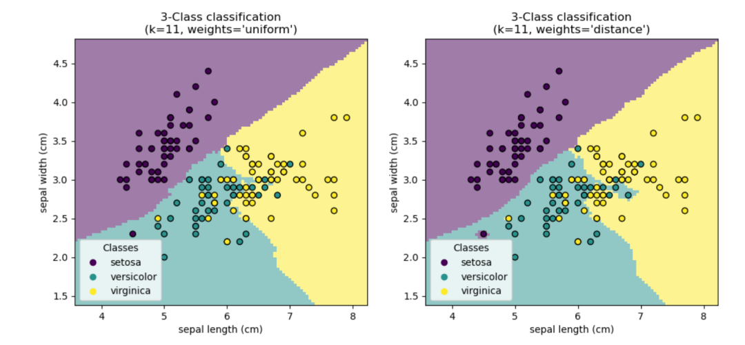
Case 2: Nearest Neighbors Classification

Scikit-learn implements two different nearest neighbor classifiers: KNeighborsClassifier, which implements learning based on the nearest neighbors of each query point, specified by an integer value defined by the user. RadiusNeighborsClassifier implements learning based on the number of neighbors within a fixed radius around each training point, specified by a floating-point value defined by the user.

In cases of uneven sampling of data, RadiusNeighborsClassifier based on radius neighbors may be a better choice. The user specifies a fixed radius to use fewer nearest neighbors for classification in sparser neighborhoods. In high-dimensional parameter spaces, this method becomes less effective due to the so-called “curse of dimensionality”.

>>> X = [[0], [3], [1]]
>>> from sklearn.neighbors import NearestNeighbors
>>> neigh = NearestNeighbors(n_neighbors=2)
>>> neigh.fit(X)
NearestNeighbors(n_neighbors=2)
>>> A = neigh.kneighbors_graph(X)
>>> A.toarray()
array([[1., 0., 1.],
       [0., 1., 1.],
       [1., 0., 1.]])

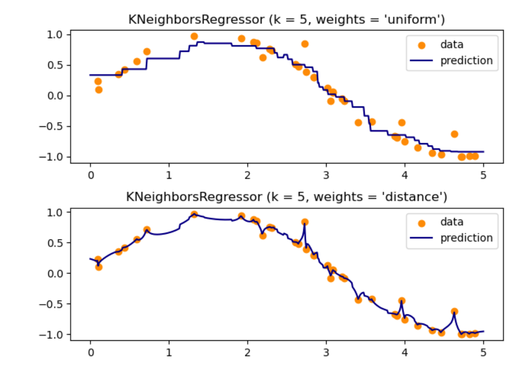
Case 3: Nearest Neighbors Regression

Scikit-learn implements two different neighbor regressors: KNeighborsRegressor, which implements learning based on the nearest neighbors of each query point, specified by an integer value defined by the user. RadiusNeighborsRegressor implements learning based on neighbors within a fixed radius around the query point, specified by a floating-point value defined by the user.

>>> X = [[0], [1], [2], [3]]
>>> y = [0, 0, 1, 1]
>>> from sklearn.neighbors import KNeighborsRegressor
>>> neigh = KNeighborsRegressor(n_neighbors=2)
>>> neigh.fit(X, y)
KNeighborsRegressor(...)
>>> print(neigh.predict([[1.5]]))
[0.5]

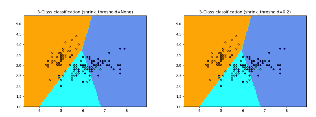
Case 4: Nearest Centroid Classifier

The nearest centroid classifier (NearestCentroid) is a simple algorithm that represents each class by the centroid of its members. In practice, this makes it similar to the label update phase of the KMeans algorithm. It also has no parameters to choose, making it a good baseline classifier. However, it may perform poorly in cases of non-convex classes or classes with significantly different variances, as it assumes equal variance across all dimensions.

>>> from sklearn.neighbors import NearestCentroid
>>> import numpy as np
>>> X = np.array([[-1, -1], [-2, -1], [-3, -2], [1, 1], [2, 1], [3, 2]])
>>> y = np.array([1, 1, 1, 2, 2, 2])
>>> clf = NearestCentroid()
>>> clf.fit(X, y)
NearestCentroid()
>>> print(clf.predict([[-0.8, -1]]))
[1]

Case 5: Nearest Neighbors Transformer

Many of scikit-learn’s estimators rely on nearest neighbor methods, including some classifiers and regressors, such as KNeighborsClassifier and KNeighborsRegressor, as well as some clustering methods like DBSCAN and SpectralClustering, and some manifold embedding methods like TSNE and Isomap.

First, precomputed graphs can be reused multiple times, for example, when tuning the parameters of estimators. This can be done manually by the user or by utilizing the caching feature of scikit-learn pipelines:

>>> import tempfile
>>> from sklearn.manifold import Isomap
>>> from sklearn.neighbors import KNeighborsTransformer
>>> from sklearn.pipeline import make_pipeline
>>> from sklearn.datasets import make_regression
>>> cache_path = tempfile.gettempdir()  # we use a temporary folder here
>>> X, _ = make_regression(n_samples=50, n_features=25, random_state=0)
>>> estimator = make_pipeline(
...     KNeighborsTransformer(mode='distance'),
...     Isomap(n_components=3, metric='precomputed'),
...     memory=cache_path)
>>> X_embedded = estimator.fit_transform(X)
>>> X_embedded.shape
(50, 3)

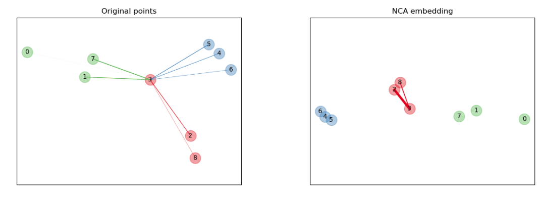
Case 6: Neighborhood Components Analysis

Neighborhood Components Analysis (NCA, Neighborhood Components Analysis) is a distance metric learning algorithm designed to improve the accuracy of nearest neighbor classification compared to standard Euclidean distance. The algorithm directly maximizes a random variant of the leave-one-out k-nearest neighbors (KNN) score on the training set. It can also learn a low-dimensional linear projection of the data for visualization and fast classification.

>>> from sklearn.neighbors import (NeighborhoodComponentsAnalysis,
... KNeighborsClassifier)
>>> from sklearn.datasets import load_iris
>>> from sklearn.model_selection import train_test_split
>>> from sklearn.pipeline import Pipeline
>>> X, y = load_iris(return_X_y=True)
>>> X_train, X_test, y_train, y_test = train_test_split(X, y,
... stratify=y, test_size=0.7, random_state=42)
>>> nca = NeighborhoodComponentsAnalysis(random_state=42)
>>> knn = KNeighborsClassifier(n_neighbors=3)
>>> nca_pipe = Pipeline([('nca', nca), ('knn', knn)])
>>> nca_pipe.fit(X_train, y_train)
Pipeline(...)
>>> print(nca_pipe.score(X_test, y_test))
0.96190476...

# Competition Exchange Group Invitation #

Daily large models, algorithm competitions, and dry goods information