Keras Implementation of RNN-LSTM for Bitcoin and Ethereum Price Prediction

How to predict Bitcoin and Ethereum price with RNN-LSTM in Keras

How to predict Bitcoin and Ethereum price in Keras using RNN-LSTM

2017 was a great year for both AI and Cryptocurrency. There have been many studies and breakthroughs in the field of artificial intelligence, and it is one of the most popular technologies today, and it will become even more popular in the future. As for cryptocurrencies, I personally did not see them becoming mainstream in 2017. It was a massive bull market, and there will be some crazy returns on investments in cryptocurrencies like Bitcoin, Ethereum, Litecoin, Ripple, etc.

I started to delve into the details of machine learning technologies at the beginning of 2017, and like many other ML experts and enthusiasts, I applied these technologies to the cryptocurrency market, which is very enticing. The interesting part is that ML and Deep Learning models can be used in various ways for the stock market or in our case, the cryptocurrency market.

I found that building a single-point prediction model can be an excellent starting point for exploring time series deep learning (like price data). Of course, it does not end here, as there is always room for improvement and the possibility of adding more input data. My favorite is to use Deep Reinforcement Learning as an automatic trading agent. This is also what I am currently researching, however, learning to use LSTM networks and building a good prediction model will be the first step.

Prerequisites and Development Environment

Assuming you already have some programming skills in Python and basic knowledge of machine learning, especially deep learning. If not, please check this article for a quick overview. (link)

https://medium.freecodecamp.org/want-to-know-how-deep-learning-works-heres-a-quick-guide-for-everyone-1aedeca88076

I chose the Google Colab as the development environment. I chose Colab because of the simplicity of setting up the environment and the use of free GPU, which makes the training time very important. Here is how to set up and use Colab in Google Drive. You can find my complete Colab Notebook on GitHub. (link)

https://github.com/SiaFahim/lstm-crypto-predictor/blob/master/lstm_crypto_price_prediction.ipynb

If you wish to set up an AWS environment, I also wrote a tutorial on how to set up an AWS instance using Docker on GPU earlier. The link is here. (link)

https://towardsdatascience.com/how-to-set-up-deep-learning-machine-on-aws-gpu-instance-3bb18b0a2579

I will use the Keras library with TensorFlow backend to build the model and train it on historical data.

What is a Recurrent Neural Network?

To explain recurrent neural networks, let’s first go back to a simple perceptron network with one hidden layer. This type of network can handle simple classification problems well. By adding more hidden layers, the network will be able to infer more complex patterns from our input data and improve prediction accuracy. However, these types of networks are suitable for tasks independent of history, where the order of historical tasks is irrelevant. For example, image classification, where previous samples in the training set do not affect the next sample. In other words, perceptrons have no memory of the past. The same goes for convolutional neural networks, which are a more complex architecture of perceptrons designed for image recognition.

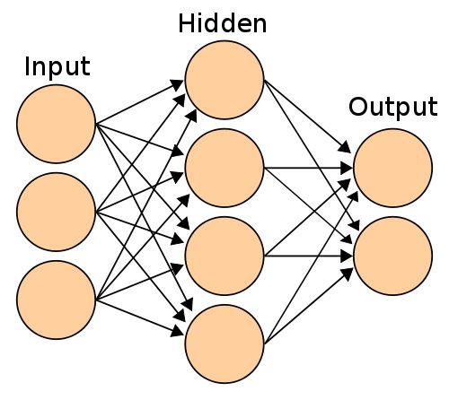
A simple perceptron neural network with one hidden layer and two outputs

RNNs are a type of neural network that addresses the past memory problem of perceptrons by cyclically inputting the current moment’s data and the previous moment’s hidden state simultaneously.

Let me explain this: each time a new sample enters, the network forgets the sample from the previous step. One way to solve time series problems is to feed the previous input sample along with the current sample, so our network can know what happened before, but this way we cannot capture the complete historical record of the time series before the previous step. A better way is to obtain the hidden layer (the weight matrix of the hidden layer) from the previous input sample and input it into our network along with the current input sample.

I consider the hidden layer’s weight matrix as the network’s mental state. If we look at it this way, the hidden layer has captured past time information in the form of the weight distribution of all neurons, which more richly represents the past of the network. The image below from Colah’s blog illustrates the principle of RNN very well.

When Xt arrives, the hidden state from Xt-1 will be concatenated with Xt and used as the input to the network at time t. This process will be repeated for every sample in the time series.

I will try to express it simply. If you want to delve deeper into RNNs, there are many resources available. Here are some good resources about RNN:

Introduction to RNNs

Recurrent Neural Networks for Beginners

The Unreasonable Effectiveness of Recurrent Neural Networks

The links are:

http://www.wildml.com/2015/09/recurrent-neural-networks-tutorial-part-1-introduction-to-rnns/

https://medium.com/@camrongodbout/recurrent-neural-networks-for-beginners-7aca4e933b82

http://karpathy.github.io/2015/05/21/rnn-effectiveness/

What is Long Short-Term Memory (LSTM)

Before telling you what LSTM is, let’s first look at the biggest problem with RNNs. So far, everything looks good until we train the samples via backpropagation. As the gradients of the training samples are backpropagated through the network, they become weaker, and when they reach those neurons representing older data points in our time series, they cannot be adjusted correctly. This problem is known as the vanishing gradient. LSTM units are a type of RNN that stores important information about the past and forgets non-important parts. This way, when the gradient is backpropagated, it is not consumed by unnecessary information.

When you read a book, you often review what you read after finishing a chapter. While you can remember the content of the previous chapter, you may not be able to remember all the important points about it. One way to solve this problem is to emphasize and record those important points and ignore the explanations that are not important to the topic. Christopher Olah’s Understanding LSTM Networks is an important resource for understanding LSTM in depth.

http://colah.github.io/posts/2015-08-Understanding-LSTMs/

Start Coding

First, we will import the libraries we need for our project.

import gc
import datetime
import pandas as pd
import numpy as np
import matplotlib.pyplot as plt

import keras
from keras.models import Sequential
from keras.layers import Activation, Dense
from keras.layers import LSTM
from keras.layers import Dropout

Historical Data

I used historical data from www.coinmarketcap.com, and you can use other data, but I think this data is very suitable for this article. We will obtain daily price data for Bitcoin. However, in the Colab notebook, you will also see the code for Ethereum. I wrote the code in such a way that it can be reused for other cryptocurrencies.

Now let’s write a function to get market data.

def get_market_data(market, tag=True):
  """
market: the full name of the cryptocurrency as spelled on coinmarketcap.com. 
eg.: 'bitcoin'
tag: eg.: 'btc', if provided it will add a tag to the name of every column.
  returns: panda DataFrame
This function will use the coinmarketcap.com url for provided coin/token 
page. 
Reads the OHLCV and Market Cap. Converts the date format to be readable. 
Makes sure that the data is consistant by converting non_numeric values to 
a number very close to 0. And finally tags each columns if provided.
  """
  market_data = pd.read_html("https://coinmarketcap.com/currencies/" + 
  market + "/historical-data/?start=20130428&end="+time.strftime("%Y%m%d"), 
flavor='html5lib')[0]
  market_data = market_data.assign(Date=pd.to_datetime(market_data['Date']))  
  market_data['Volume'] = (pd.to_numeric(market_data['Volume'], 
errors='coerce').fillna(0))
  if tag:
    market_data.columns = [market_data.columns[0]] + [tag + '_' + i for i in
market_data.columns[1:]]
  return market_data

Now let’s get the Bitcoin data and load it into the variable ”’btc_data”’ and display the first row of our data.

btc_data = get_market_data("bitcoin", tag='BTC')
btc_data.head()

Market data for BTC

Let’s take a look at the ‘Close’ price of Bitcoin and the daily trading volume over time.

show_plot(btc_data, tag='BTC')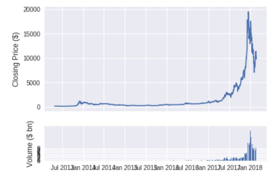

Data Preparation

Building any deep learning model involves a significant amount of preparing our data for training or prediction in the neural network. This step is called preprocessing, and depending on the type of data we are using, it may involve multiple steps. In our case, we will do the following as part of our preprocessing:

Data cleaning, filling in missing data points

Combining multiple data channels. Bitcoin and Ethereum in one data frame.

Calculating price volatility and adding it as a new column

Removing unnecessary columns

Sorting our data in ascending order by date

Splitting data for training and testing

Creating input samples and normalizing between 0 and 1

Creating target outputs for the training and testing sets and normalizing them to between 0-1

Converting our data to numpy arrays for our model to use

The data cleaning part has already been completed in the first function where we load the data. You can find the necessary functions to complete the tasks mentioned above below:

def merge_data(a, b, from_date=merge_date):
  """
  a: first DataFrame
  b: second DataFrame
  from_date: includes the data from the provided date and drops the any data 
before that date.
  returns merged data as Pandas DataFrame
  """
  merged_data = pd.merge(a, b, on=['Date'])
  merged_data = merged_data[merged_data['Date'] >= from_date]
  return merged_data


def add_volatility(data, coins=['BTC', 'ETH']):
  """
  data: input data, pandas DataFrame
  coins: default is for 'btc and 'eth'. It could be changed as needed
  This function calculates the volatility and close_off_high of each given 
  coin in 24 hours, 
  and adds the result as new columns to the DataFrame.
  Return: DataFrame with added columns
  """
  for coin in coins:
    # calculate the daily change
    kwargs = {coin + '_change': lambda x: (x[coin + '_Close'] - x[coin + 
    '_Open']) / x[coin + '_Open'], coin + '_close_off_high': lambda x: 
    2*(x[coin + '_High'] - x[coin + '_Close']) / (x[coin + '_High'] - 
    x[coin + '_Low']) - 1, coin + '_volatility': lambda x: (x[coin + 
    '_High'] - x[coin + '_Low']) / (x[coin + '_Open'])}
    data = data.assign(**kwargs)
  return data


def create_model_data(data):
  """
  data: pandas DataFrame
This function drops unnecessary columns and reverses the order of DataFrame
based on decending dates.
  Return: pandas DataFrame
  """
  #data = data[['Date']+[coin+metric for coin in ['btc_', 'eth_'] for metric 
in ['Close','Volume','close_off_high','volatility']]]
  data = data[['Date']+[coin+metric for coin in ['BTC_', 'ETH_'] for metric 
in ['Close','Volume']]]
  data = data.sort_values(by='Date')
  return data


def split_data(data, training_size=0.8):
  """
  data: Pandas Dataframe
  training_size: proportion of the data to be used for training
  This function splits the data into training_set and test_set based on the 
given training_size
  Return: train_set and test_set as pandas DataFrame
  """
  return data[:int(training_size*len(data))], 
data[int(training_size*len(data)):] 


def create_inputs(data, coins=['BTC', 'ETH'], window_len=window_len):
  """
  data: pandas DataFrame, this could be either training_set or test_set
  coins: coin datas which will be used as the input. Default is 'btc', 'eth'
  window_len: is an intiger to be used as the look back window for creating 
a single input sample.
  This function will create input array X from the given dataset and will 
  normalize 'Close' and 'Volume' between 0 and 1
  Return: X, the input for our model as a python list which later needs to 
  be converted to numpy array.
  """
  norm_cols = [coin + metric for coin in coins for metric in ['_Close', 
'_Volume']]
  inputs = []
  for i in range(len(data) - window_len):
    temp_set = data[i:(i + window_len)].copy()
    inputs.append(temp_set)
    for col in norm_cols:
      inputs[i].loc[:, col] = inputs[i].loc[:, col] / inputs[i].loc[:, col].
      iloc[0] - 1  
  return inputs


def create_outputs(data, coin, window_len=window_len):
  """
  data: pandas DataFrame, this could be either training_set or test_set
  coin: the target coin in which we need to create the output labels for
  window_len: is an intiger to be used as the look back window for creating 
a single input sample.
  This function will create the labels array for our training and validation 
and normalize it between 0 and 1
  Return: Normalized numpy array for 'Close' prices of the given coin
  """
  return (data[coin + '_Close'][window_len:].values / data[coin + '_Close']
  [:-window_len].values) - 1


def to_array(data):
  """
  data: DataFrame
  This function will convert list of inputs to a numpy array
  Return: numpy array
  """
  x = [np.array(data[i]) for i in range (len(data))]
  return np.array(x)

Below is the code for plotting and creating date labels:

def show_plot(data, tag):
    fig, (ax1, ax2) = plt.subplots(2, 1, gridspec_kw={'height_ratios': 
    [3, 1]})
    ax1.set_ylabel('Closing Price ($)', fontsize=12)
    ax2.set_ylabel('Volume ($ bn)', fontsize=12)
    ax2.set_yticks([int('%d000000000' % i) for i in range(10)])
    ax2.set_yticklabels(range(10))
    ax1.set_xticks([datetime.date(i, j, 1) for i in range(2013, 2019) for j 
in [1, 7]])
    ax1.set_xticklabels('')
    ax2.set_xticks([datetime.date(i, j, 1) for i in range(2013, 2019) for j 
in [1, 7]])
    ax2.set_xticklabels([datetime.date(i, j, 1).strftime('%b %Y') for i in 
range(2013, 2019) for j in [1, 7]])
    ax1.plot(data['Date'].astype(datetime.datetime), data[tag + '_Open'])
    ax2.bar(data['Date'].astype(datetime.datetime).values, data[tag + 
    '_Volume'].values)
    fig.tight_layout()
    plt.show()


def date_labels():
    last_date = market_data.iloc[0, 0]
    date_list = [last_date - datetime.timedelta(days=x) for x in 
range(len(X_test))]
    return [date.strftime('%m/%d/%Y') for date in date_list][::-1]


def plot_results(history, model, Y_target, coin):
    plt.figure(figsize=(25, 20))
    plt.subplot(311)
    plt.plot(history.epoch, history.history['loss'], )
    plt.plot(history.epoch, history.history['val_loss'])
    plt.xlabel('Number of Epochs')
    plt.ylabel('Loss')
    plt.title(coin + ' Model Loss')
    plt.legend(['Training', 'Test'])

    plt.subplot(312)
    plt.plot(Y_target)
    plt.plot(model.predict(X_train))
    plt.xlabel('Dates')
    plt.ylabel('Price')
    plt.title(coin + ' Single Point Price Prediction on Training Set')
    plt.legend(['Actual', 'Predicted'])

    ax1 = plt.subplot(313)
    plt.plot(test_set[coin + '_Close'][window_len:].values.tolist())
    plt.plot(((np.transpose(model.predict(X_test)) + 1) * test_set[coin + 
    '_Close'].values[:-window_len])[0])
    plt.xlabel('Dates')
    plt.ylabel('Price')
    plt.title(coin + ' Single Point Price Prediction on Test Set')
    plt.legend(['Actual', 'Predicted'])

    date_list = date_labels()
    ax1.set_xticks([x for x in range(len(date_list))])
    for label in ax1.set_xticklabels([date for date in date_list], 
rotation='vertical')[::2]:
        label.set_visible(False)

    plt.show()

Here we will call the above functions to create the final dataset for our model.

train_set = train_set.drop('Date', 1)
test_set = test_set.drop('Date', 1)
X_train = create_inputs(train_set)
Y_train_btc = create_outputs(train_set, coin='BTC')
X_test = create_inputs(test_set)
Y_test_btc = create_outputs(test_set, coin='BTC')
Y_train_eth = create_outputs(train_set, coin='ETH')
Y_test_eth = create_outputs(test_set, coin='ETH')
X_train, X_test = to_array(X_train), to_array(X_test)

Now we will build our LSTM-RNN model. In this model, I used 3 layers of LSTM with 512 neurons each, followed by a Dropout layer with a probability of 0.25 to prevent overfitting, and finally a Dense layer produces our output.

def build_model(inputs, output_size, neurons, activ_func=activation_function
, dropout=dropout, loss=loss, optimizer=optimizer):
  """
  inputs: input data as numpy array
  output_size: number of predictions per input sample
  neurons: number of neurons/ units in the LSTM layer
  active_func: Activation function to be used in LSTM layers and Dense layer
  dropout: dropout ration, default is 0.25
  loss: loss function for calculating the gradient
  optimizer: type of optimizer to backpropagate the gradient
  This function will build 3 layered RNN model with LSTM cells with dripouts 
after each LSTM layer 
and finally a dense layer to produce the output using keras' sequential 
model.
  Return: Keras sequential model and model summary
  """
  model = Sequential()
  model.add(LSTM(neurons, return_sequences=True, 
input_shape=(inputs.shape[1], inputs.shape[2]), activation=activ_func))
  model.add(Dropout(dropout))
  model.add(LSTM(neurons, return_sequences=True, activation=activ_func))
  model.add(Dropout(dropout))
  model.add(LSTM(neurons, activation=activ_func))
  model.add(Dropout(dropout))
  model.add(Dense(units=output_size))
  model.add(Activation(activ_func))
  model.compile(loss=loss, optimizer=optimizer, metrics=['mae'])
  model.summary()
  return model

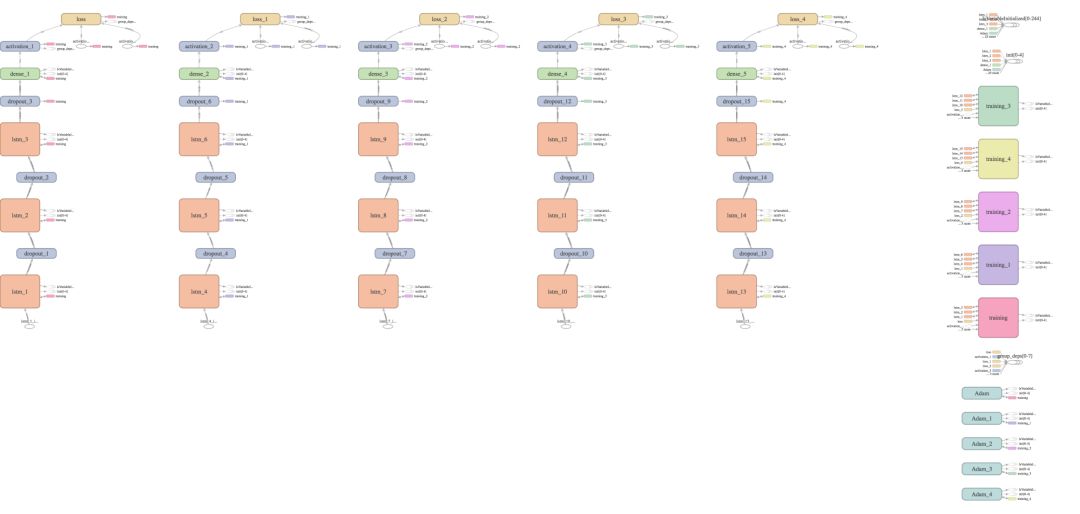
I used ‘tanh’ as my activation function, MSE as my loss, and ‘adam’ as my optimizer. I recommend trying different choices for each part and see how they affect the model’s performance.

This is our model summary:

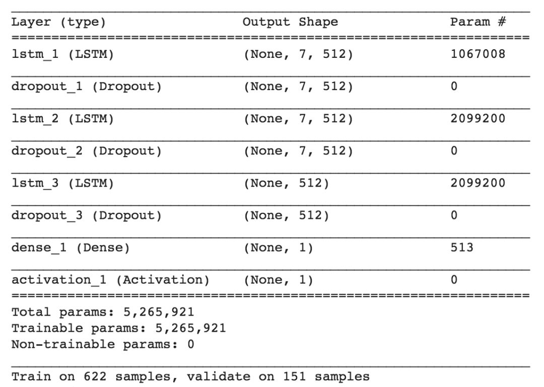
I have declared the hyperparameters at the start of the code to make it easier to change them from one place for different variants. Here are my hyperparameters:

neurons = 512                 
activation_function = 'tanh'  
loss = 'mse'                  
optimizer="adam"              
dropout = 0.25                 
batch_size = 12               
epochs = 53                   
window_len = 7                
training_size = 0.8
merge_date = '2016-01-01'

Now it’s time to train our model on the collected data

# clean up the memory
gc.collect()
# random seed for reproducibility
np.random.seed(202)
# initialise model architecture
btc_model = build_model(X_train, output_size=1, neurons=neurons)
# train model on data
btc_history = btc_model.fit(X_train, Y_train_btc, epochs=epochs, 
batch_size=batch_size, verbose=1, validation_data=(X_test, Y_test_btc), 
shuffle=False)

The above code may take some time to complete, depending on your computing power, and once done, your training model is also complete 🙂

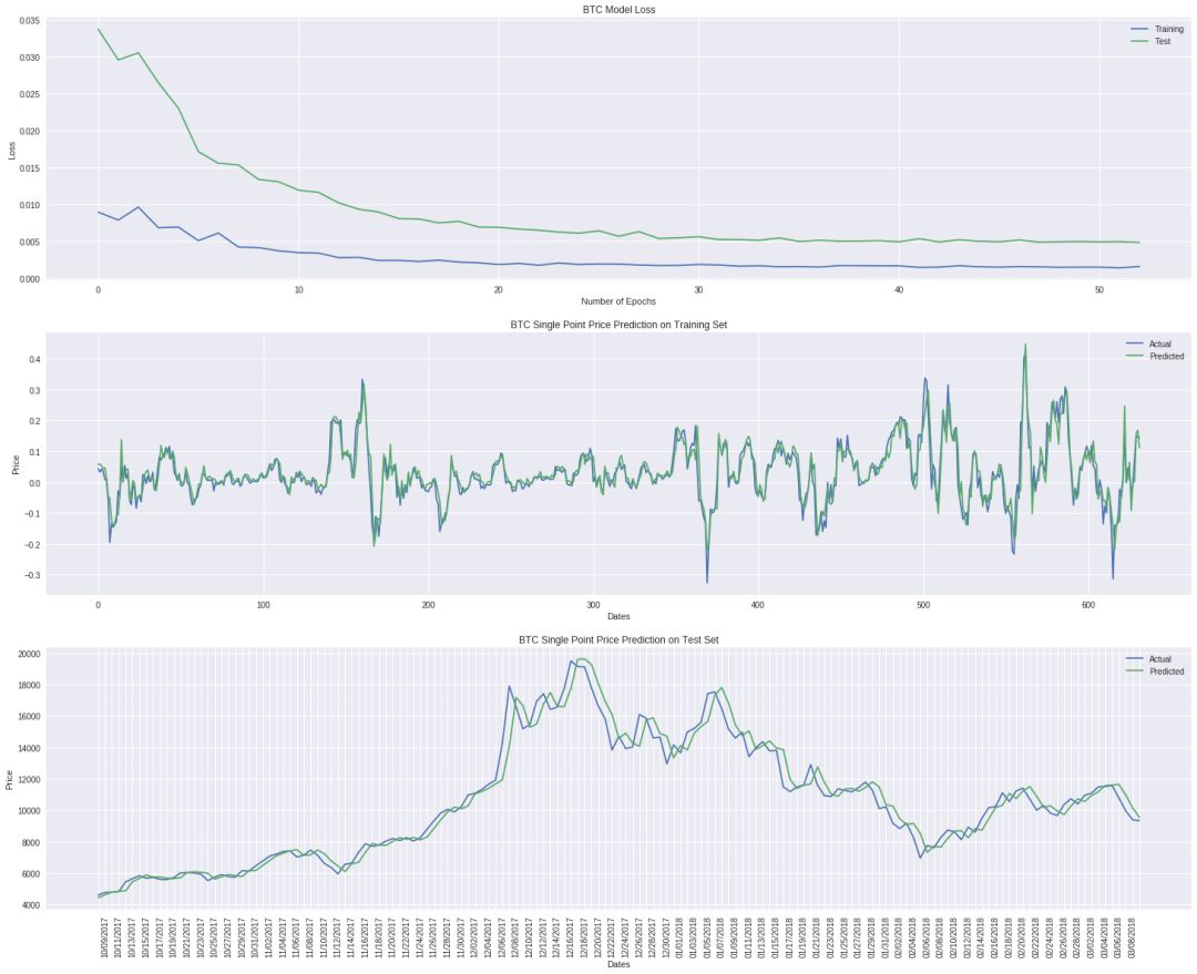
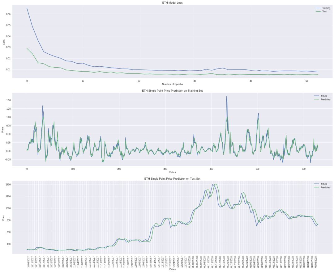
Let’s take a look at the results for BTC and ETH.

References Literature

https://medium.com/@siavash_37715/how-to-predict-bitcoin-and-ethereum-price-with-rnn-lstm-in-keras-a6d8ee8a5109

ttps://dashee87.github.io/deep%20learning/python/predicting-cryptocurrency-prices-with-deep-learning/

Code link:

https://github.com/SiaFahim/lstm-crypto-predictor/blob/master/lstm_crypto_price_prediction.ipynb

h

-END-

Special Knowledge