Introduction to GAN in 9102

“ This article mainly introduces the recent developments and representative works of GAN (Generative Adversarial Networks) in distribution discrepancy measurement, IPM and regularization, dual learning, conditioning and control, resolution enhancement, evaluation metrics, etc. It is hoped to help those who have not followed GAN-related work before ～“

Author:Zongheng

Source: Zhihu Column Machine Learning

Editor: happyGirl

Recently, under the guidance of my mentor, I conducted some research on GAN + GCN/video. I must say that GAN has been popular for such a long time and still has strong vitality in the intersection fields of graph convolution and video analysis. There are still many problems to solve when 1+1=2. During my research, I first tried some basic models and recorded some of the representative ones. I will continue to record GAN + GCN / GAN + video and my ongoing implementation of pytorch gan zoo when I have time.

In 9102, the goal of embedding everything has basically been achieved, representation learning has received widespread attention, and generative learning is in full swing. In my recent research, I found that there are few remaining bonding works in the intersection of 1+1=2. However, even after 1+1=2, there are still some minor problems related to task characteristics. To solve the minor problems in my field, I summarized and reproduced the classic GAN networks, hoping to help those who have not followed GAN-related work before ～

Guide

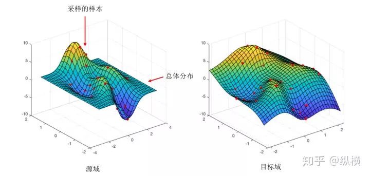
Many existing machine learning tasks can be summarized as domain transform, converting data from the source domain to the target domain, such as generating images from text, generating the next frame from the previous one, converting one style to another, etc. Existing neural network modules have been able to help us map source data to any target size, while traditional loss functions such as MSE, MAE, Huber Loss, etc., can also measure the difference between generated samples and target domain samples.

However, models constructed in this way (e.g., Auto Encoder) often become less satisfactory after BP.

During the research process, some works found that these traditional loss functions can only roughly calculate gradients based on the average error of all pixels during the NN update process, leading to many marginal distributions and local differences not being learned.

As shown in the figure above, the number of pixels modified in the two generated images is the same based on the original image, so their MSE error is the same. However, according to common sense, the second image obviously does not conform to the pattern of 0. A good loss function should assign a larger MSE to the second generated image.

Based on this, the GAN network proposes a learnable loss function, namely the discriminator, which adaptively measures the difference between the two overall distributions, that is, continuous probability distributions. (Unlike traditional fixed loss functions such as MSE, MAE, Huber Loss, which measure the difference between two samples, i.e., discrete probability distributions).

In the derivation process, most works are based on the theory of Bayesian statistics, maximizing the likelihood of the generated domain and target domain.

I personally believe that a truly viable research direction does not necessarily have good performance, but at least should be able to split into different sub-problems, each blooming and bearing fruit. If everyone is stacking and modifying the module on one problem, then this research direction may only be fleeting. GAN, as a topic that is still thriving in 2019, has optimization directions in CV that can be divided into the following 6 categories:

1. Measurement of Distribution Differences

Improving the measurement of the difference between generated distribution and target distribution, enhancing the accuracy and diversity of generation.

2. IPM and Regularization

Truncating gradients and adding regularization to improve the stability of GAN convergence.

3. Dual Learning

Utilizing cyclic consistency, adding constraints between the source domain and the reconstruction domain to make full use of data.

4. Conditioning and Control

Integrating known conditions to control the features of the generation process and results.

5. Efforts to Improve Resolution

Traditional GAN networks are relatively blurry when generating large images, and some works have studied how to improve the resolution of generated images.

6. Evaluation Metrics

Measuring the generation effects of different GANs.

1. Measurement of Distribution Differences

In the previous text, we mentioned that the essential goal of GAN is to make the generated distribution as close as possible to the target distribution. However, how should we measure the difference between the two probability distributions?

GAN

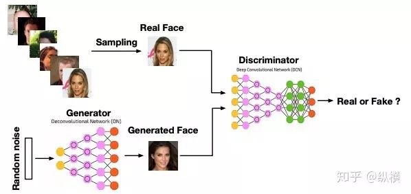
Goodfellow first proposed the minimax game, opening the chapter of GAN. GAN needs to train two models simultaneously, one that captures the data distribution (the generator) and one that estimates whether the data is real (the discriminator). The training goal of the generator is to maximize the probability of the discriminator making a mistake, that is, by optimizing the generated distribution, making the discriminator mistakenly think that the generated fake samples are real. The training goal of the discriminator is to minimize the probability of making a mistake, that is, to find the fake samples generated by the generator; the loss can be expressed as:

In the implementation process, the discriminator and generator of GAN are often alternately optimized (or 5:1), and the optimization objectives of the discriminator and generator can be written as:

Paper: arxiv (https://arxiv.org/abs/1406.2661)

Code: github (https://github.com/eriklindernoren/PyTorch-GAN/blob/master/implementations/gan/gan.py)

LSGAN

LSGAN encodes generated samples and real samples as and , and uses mean squared error to replace GAN’s logistic loss:

Experiments show that LSGAN can partly solve the problems of unstable GAN training and poor quality of generated images. However, the mean squared error excessively punishes outliers, which may lead to overfitting to real samples and reduce the diversity of generated results.

Paper: arxiv Code: [ github ](https://link.zhihu.com/?target=https%3A//github.com/LynnHo/DCGAN-LSGAN-WGAN-GP-DRAGAN-Pytorch/blob/master/v0/train_celeba_lsgan.py)

f-GAN

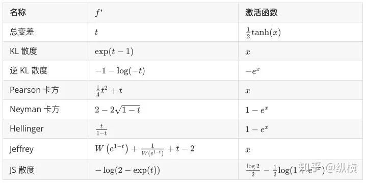
f-GAN further expands the loss function of GAN, believing that the JS divergence used by GAN and the Chi-squared divergence used by LSGAN are both special cases of divergence, and other different distances or divergences can also be used to measure the real distribution and generated distribution. Based on this, f-GAN designs a set of losses obtained from different divergences:

Where, can be replaced by various expressions according to different divergences; since has requirements on the range of the discriminator, the activation function of the output layer of the discriminator also needs to be replaced:

Paper: arxiv (https://arxiv.org/abs/1606.00709)

Code: github(https://github.com/shayneobrien/generative-models/blob/master/src/f_gan.py)

EBGAN

f-GAN culminates from the divergence perspective, while EBGAN views the discriminator as an energy function, serving as a trainable loss function. This energy function considers areas close to the real distribution as low-energy areas and areas far from the real distribution as high-energy areas. The generator will try to generate fake samples with the minimum energy. From this perspective, the network structure and loss function of the generator become more flexible and variable. EBGAN proposes to use an autoencoder structure, replacing the classification results of the classifier with reconstruction error:

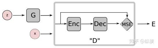
That is, . In designing the loss function, to stabilize the energy model, the author adds a margin value:

Paper: arxiv(https://arxiv.org/abs/1609.03126)

Code: github(https://github.com/eriklindernoren/PyTorch-GAN/blob/master/implementations/ebgan/ebgan.py)

2. IPM and Regularization

Many times, due to adversarial learning, the convergence of GAN is not ideal. IPM (Integral Probability Metric) transforms the output of the discriminator from probability to real numbers and effectively prevents the discriminator from optimizing too early, leading to the problem of vanishing gradients for the generator through regularization that limits the gradients within a certain range.

WGAN

After analyzing the reasons for the unstable convergence of GAN, WGAN believes that the difficulty of controlling the gradients during discriminator training is the main culprit for the unstable convergence of GAN. If the discriminator is trained too well, the gradient of the generator vanishes, and the loss becomes difficult to decrease; if the discriminator is poorly trained, the gradient of the generator is inaccurate, and the loss runs all over the place. Only by balancing the discriminator and generator in a zero-sum game can it work.

WGAN made the following modifications:

1. The last layer of the discriminator cancels the sigmoid

2. Gradient clipping is applied to the discriminator, limiting the gradient values within the interval.

3. Using RMSProp or SGD and optimizing at a lower learning rate

The loss function can be expressed as:

acts to smooth out the drastic changes of , which can be expressed as:

In implementation, this means limiting the gradient values within the interval.

Paper: arxiv(https://arxiv.org/abs/1701.07875) Code: github(https://github.com/Zeleni9/pytorch-wgan/blob/master/models/wgan_clipping.py)

WGAN-GP

Shortly after WGAN was proposed, the author of WGAN optimized WGAN by replacing gradient clipping (weight clipping) with gradient penalty, proposing WGAN-gp with gradient penalty.

Paper: arxiv(https://arxiv.org/abs/1704.00028) Code: github(https://github.com/caogang/wgan-gp/blob/master/gan_cifar10.py)

BEGAN

BEGAN further combines the ideas of WGAN and EBGAN. On the one hand, BEGAN uses autoencoders and reconstruction error to measure the difference between generated samples and real samples:

On the other hand, BEGAN trains a hyperparameter to balance the optimization speed of the discriminator and generator:

Paper: arxiv(https://arxiv.org/abs/1703.10717) Code: github(https://github.com/shayneobrien/generative-models/blob/master/src/be_gan.py)

3. Dual Learning

Some works expand the generation-recognition process of GAN into a generation-recognition and reconstruction-recognition process through dual learning, making fuller use of information from the source domain and target domain. DaulGAN, CycleGAN, and DiscoGAN have similar network structures, but the differences in motivation are interesting:

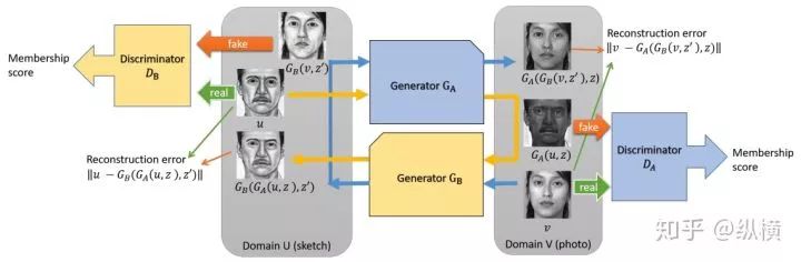
DaulGAN

DaulGAN proposes that converting the source distribution to the target distribution and converting the target distribution back to the source distribution is a dual problem that can be optimized collaboratively.

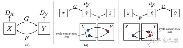
CycleGAN

CycleGAN proposes the principle of cycle consistency, which means that an image should be able to return to its original image after being mapped to another type of image and then inversely mapped.

Paper: arxiv(https://arxiv.org/abs/1703.10593) Code: github(https://github.com/aitorzip/PyTorch-CycleGAN/blob/master/models.py)

DiscoGAN

To learn the mapping between different domains, DiscoGAN first thought of adding a second generator and a reconstruction loss term to compare real images and reconstructed images.

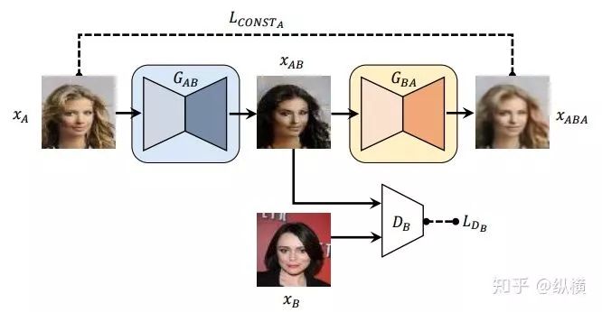
However, the model designed this way is a unidirectional mapping and cannot learn how to map back from the target domain to the source domain simultaneously. Additionally, due to the excessive punishment of outliers by MSE, the model may have mode collapse issues, making only minor modifications to the source image. Therefore, the author further proposed the bidirectional mapping DiscoGAN:

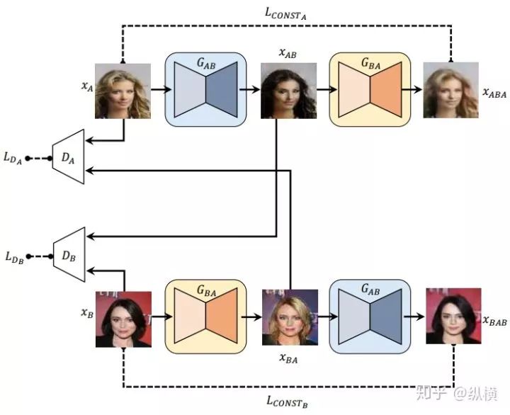
Paper: arxiv(https://arxiv.org/abs/1703.05192) Code: github(https://github.com/carpedm20/DiscoGAN-pytorch/blob/master/models.py)

4. Conditioning and Control

The generated samples of GAN are uncontrollable. Conditional GAN (cGAN) controls the generation process of samples by adding prior/conditions, guiding the generated samples to meet certain features.

cGAN

Through GAN, distributions close to the target distribution can be generated, such as generating digits from 0 to 9. However, we cannot intervene in the process of traditional GAN generating distributions, such as specifying to generate the digit 1. Therefore, cGAN changes the probability distribution in GAN to a conditional probability:

Specifically, this means concatenating the known condition vector in the inputs of both the generator and discriminator:

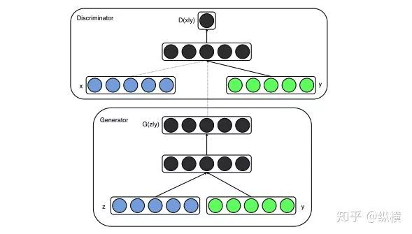
In the figure, represents noise sampled from a normal distribution; represents samples sampled from the real distribution; represents the condition vector, such as the one-hot encoding of sample labels. When the discriminator discriminates the generated samples, it will judge based on the conditions, thus forcing the generator to reference the condition vector to generate samples.

Paper: arxiv(https://arxiv.org/abs/1411.1784) Code: github(https://github.com/eriklindernoren/PyTorch-GAN/blob/master/implementations/cgan/cgan.py)

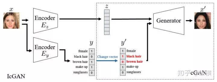
IcGAN

Initially, cGAN only used the one-hot encoding of sample labels as input to control the generation of samples at the label level. How can we change certain features of generated samples more finely? IcGAN learns the mapping from the original image to its feature vector through an encoder, and then generates the desired features by modifying some features of the feature vector as input to the generator:

ACGAN

ACGAN does not choose to directly input the condition (the category of the sample) into the discriminator, but trains the discriminator to classify the samples, meaning that the discriminator not only needs to judge the authenticity of each sample but also needs to predict the known conditions (the category of the sample, adding a classification loss).

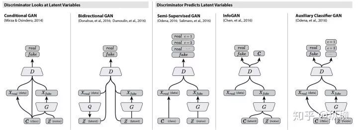
A benefit of ACGAN is that the design of the discriminator outputting conditions allows us to use models pretrained on other datasets for prior learning, thus generating clearer images and alleviating mode collapse issues. Additionally, as shown in the figure, there are other similar designs that add prior distributions to GAN, such as SemiGAN and InfoGAN, but they are quite similar.

Paper: arxiv(https://arxiv.org/abs/1610.09585) Code: github(https://github.com/eriklindernoren/PyTorch-GAN/blob/master/implementations/acgan/acgan.py)

5. Efforts to Improve Resolution

In the initial works, limited by the size of noise sampled from a normal distribution, GAN could only generate low-resolution images of 32×32. Some works have studied how to generate high-resolution images.

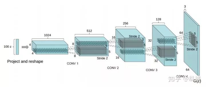
DCGAN

DCGAN was the first to introduce CNN into GAN (previously, GANs were mostly composed of fully connected layers) and proposed a CNN + GAN structure that could converge stably. Many tricks provided a foundation for subsequent research:

1. Downsampling uses convolution with stride instead of pooling

2. Upsampling uses transposed convolution instead of interpolation

3. The activation function of the discriminator uses Leaky ReLU

4. Using BatchNorm layers (Note: Not applicable in WGAN)

5. Duality between the generator and discriminator, etc.

Paper: arxiv(https://arxiv.org/abs/1511.06434) Code: github(https://github.com/eriklindernoren/PyTorch-GAN/blob/master/implementations/dcgan/dcgan.py)

SAGAN

With the deepening of research, some commonly used modules in CV combined with CNN have gradually been introduced. SAGAN proposed the introduction of Self Attention modules in both the generator and discriminator to obtain information from distant relevant areas, enhancing the clarity of generated images.

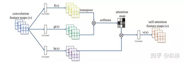
In the original implementation, Self Attention only needs to be added to the last two layers of the generator and discriminator.

Paper: arxiv(https://arxiv.org/abs/1805.08318) Code: github(https://github.com/heykeetae/Self-Attention-GAN/blob/master/sagan_models.py)

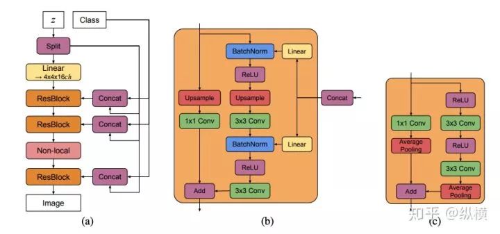
BigGAN

As available modules gradually increase, an arms race for network parameters has also gradually unfolded. BigGAN, as a milestone in the history of GAN development, achieved a leap in accuracy (128×128 resolution). Although its model is large and difficult to reproduce locally, the Self Attention, Res Block, large channel/batch, and gradient stage tricks used in BigGAN provide references for subsequent research.

Paper: arxiv(https://arxiv.org/abs/1809.11096) Code: github(https://github.com/ajbrock/BigGAN-PyTorch/blob/master/BigGANdeep.py)

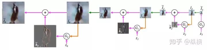
LAPGAN

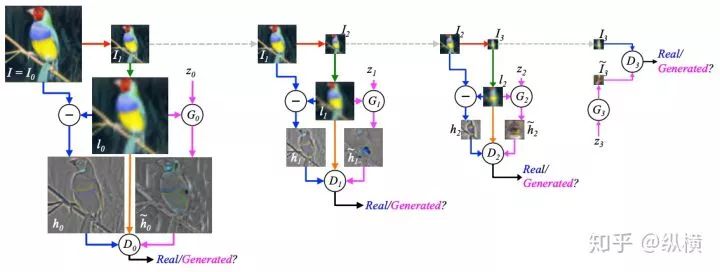
LAPGAN combines CGAN, applying iterative and hierarchical ideas to image generation. LAPGAN believes that rather than generating high-resolution images all at once, it is better to first generate low-resolution images. In the process of upsampling and increasing resolution, the generator generates the missing detail information, i.e., “residual” images, and adds them to the upsampled images to obtain higher resolution images:

During the training process, LAPGAN uses the downsampled images as prior conditions at each resolution, learning the information loss from downsampling to upsampling and generating the residuals:

Paper: arxiv(https://arxiv.org/abs/1506.05751)

Code: github (https://github.com/AaronYALai/Generative_Adversarial_Networks_PyTorch/blob/master/LAPGAN/LAPGAN.py)

6. Evaluation Metrics

The loss of the generator can measure the performance of the generated images in deceiving the discriminator, but it cannot measure the accuracy and diversity of the generated images. Therefore, in addition to subjective evaluations, objective evaluation metrics such as IS and FID have emerged in recent years (similar to PSNR for assessing image quality) to evaluate the accuracy and diversity of generated images (some students ask whether these evaluation metrics can be used as loss: these metrics only reflect certain statistical characteristics of the generated data, and cannot guide GAN optimization as loss).

IS

Inception Score, as an early evaluation metric, proposes that the results generated by GAN can be measured by two dimensions: the accuracy (classifiability) and diversity of the generated results. Taking generated images as an example, for a clear image, its probability of belonging to a certain class should be very high, while the probability of belonging to other classes should be low (it can be accurately classified by Inception v3). At the same time, if GAN can generate sufficiently diverse images, then the generated images should be evenly distributed across various categories (rather than just a few, i.e., mode collapse).

It is worth noting that the larger the IS, the better the effect of GAN.

Code: github(https://github.com/sbarratt/inception-score-pytorch/blob/master/inception_score.py)

FID

However, IS has a problem: real images are not involved in the evaluation of generated images. Therefore, FID proposes to compare generated images with real images (at the feature map level of Inception v3), achieving an evaluation of the accuracy and diversity of generated images.

It is worth noting that the smaller the FID, the better the effect of GAN.

Code: github(https://github.com/mseitzer/pytorch-fid/blob/master/fid_score.py)

Others

Both FID and IS are feature extraction-based evaluation methods; the feature map effectively describes whether certain features appear, but cannot describe the spatial relationships of these features. Therefore, in recent years, articles such as GAN dissertation and GAN and GMM have further analyzed the generation effects of GAN.

An interesting conclusion is that most GAN models currently do not significantly improve over the original GAN model; they only converge faster and more stably. Therefore, when solving cross-domain problems, I generally first use the conventional WGAN-GP for testing to get a rough baseline, then decide whether to continue in-depth research or explore task-specific issues.

Postscript

I saw a great quote that guides our scientific research (escape) and share it with everyone ～

A hierarchical structure does not mean that discipline X is “merely the application of Y.” Each new hierarchy requires completely new laws, concepts, and inductions, and like its previous hierarchy, the research process requires a lot of inspiration and creativity. Psychology is not applied biology, and biology is not applied chemistry.