Introduction to Explainable Machine Learning Methods

1. Concept

Machine learning is an important branch of artificial intelligence, focusing on improving the performance of computer systems or algorithms through learning from experience data to adapt to various environments and tasks. As machine learning becomes increasingly integrated into everyday life and widely applied, people are becoming more reliant on the critical decisions made by it. However, due to the complex structure of machine learning models, users find it difficult to intuitively understand their prediction processes, only receiving the final results, similar to a “black box”, which makes it hard to trust. This is particularly challenging for medical decision-makers, who find it difficult to conclude on patients based solely on the model’s predictions without understanding the basis of the black box model’s decisions, leading to difficulties in practical applications. Therefore, the reliability of machine learning is gaining more attention.

Explainable Machine Learning (XML) refers to methods that provide clear descriptions and understandings of machine learning models and their predictions, enabling users to better comprehend and explain the model’s prediction processes and results. Its core goal is to enhance the transparency of machine learning models, helping users answer “Why did the model make a certain prediction?” and “What factors did the model consider when making decisions?”

2. Classification

Explainable machine learning methods can be divided into two types based on different stages: Intrinsic Explainability and Post-hoc Explainability.

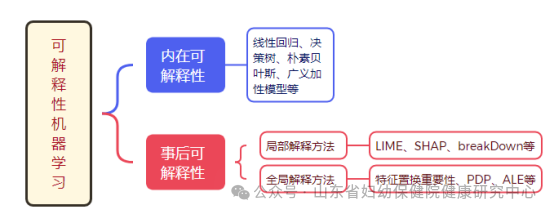
1.Intrinsic Explainability

Intrinsic explainability, also known as pre-explainability, refers to the capability of machine learning models to be understood without additional information by training simple structures that are inherently interpretable or by integrating interpretability into specific model structures. For example:

lLinear Regression: Explaining each feature’s contribution to the prediction results through the model’s coefficients;

lDecision Trees: Displaying feature importance and decision paths in a tree structure;

lNaive Bayes: Providing the contribution of each feature to the classification probability;

lGeneralized Additive Models: Visually presenting the impact of each feature through smooth function graphs.

These models inherently possess high interpretability due to their simple structures, but their performance is often limited when dealing with complex data.

2.Post-hoc Explainability

Post-hoc explainability refers to using explanation methods or constructing explanation models to explain the working mechanisms, decision behaviors, and bases of a given trained model. Post-hoc explanation methods can be divided into two categories based on their scope: local interpretation methods and global interpretation methods. Local interpretation methods explain why a model makes a certain prediction for a single sample or a group of samples, while global interpretation methods can provide general rules or statistical inferences about the overall model, understanding each variable’s impact.

(1) Examples of Local Interpretation Methods:

lLIME (Local Interpretable Model-agnostic Explanations): One of the most popular post-hoc explanation methods for black box models, proposed by Marco Ribeiro et al. in 2016, which explains a sample’s prediction result through local linear approximations of the model output. Advantages: Flexible and applicable to any model.

lSHAP (Shapley Additive Explanations): Proposed by Lundberg and Lee in 2017, based on game theory, assigning a contribution value to each feature. SHAP also averages the Shapley values of all sample variables to determine global variable importance. Advantages: Can explain both global and local feature impacts, theoretically rigorous.

lbreakDown: Proposed by Staniak et al. in 2018, similar to SHAP, which decomposes the model prediction into the incremental contributions of each feature, visually displaying each feature’s impact on the prediction results and its cumulative contribution. Advantages: Faster computation speed, more intuitive explanations.

(2) Examples of Global Interpretation Methods:

lFeature Permutation Importance: Evaluating feature importance by randomly shuffling feature values and observing changes in model performance. Advantages: Simple to use, applicable to various models.

lPartial Dependence Plot (PDP): Graphically displaying the average impact of one or more features on the model output. Characteristics: Considers the average impact of all samples on predictions, but averaging across all samples may result in positive and negative effects canceling each other out, and does not allow for correlations between variables.

lAccumulated Local Effects (ALE): Measuring the local average impact of feature value changes on model predictions, avoiding feature correlation bias, thus clearly reflecting the overall impact trend of features on predictions. Characteristics: Improves PDP, reducing the influence of feature correlations on explanations.

3. Choosing Explainable Machine Learning Methods

Due to the variety of explainable machine learning methods, it is essential to choose suitable explainability methods based on task requirements and model complexity:

1.Simple Models (e.g., regression, decision trees): Directly use model structure for explanation.

2.Complex Models (e.g., deep learning, random forests): Combine SHAP, LIME, and other methods.

3.High-risk Scenarios (e.g., healthcare, finance): Prioritize explanation methods with strong theoretical support and high transparency.

4. Implementing Explainable Machine Learning Methods

The implementation of explainable machine learning methods can be accomplished through various open-source libraries and tools, which provide a wide range of explanation techniques for different models. The main implementation tools include Python packages such as SHAP, LIME, ELI5, InterpretML, Yellowbrick, TensorBoard, etc., and R language packages like lime, shapviz, ibreakdown, which can also explain some machine learning model results.

5. Applications of Explainable Machine Learning Methods

Explainable machine learning methods have significant application value in various fields, such as:

1.Healthcare: Explaining diagnostic models or treatment recommendation systems, such as disease prediction or drug recommendations.

2.Financial Services: Evaluating the decision logic of models in credit scoring, risk analysis, and fraud detection systems.

3.Industrial Manufacturing: Analyzing models for optimizing production processes and predicting equipment failures.

4.Environmental Science: Analyzing the feature contributions of climate change models and pollution prediction models.

5.Autonomous Driving and Traffic: Evaluating the reliability of decision models for path planning and obstacle detection.

6.Public Policy and Social Sciences: Assessing the fairness and influencing factors of policy decision models.

In summary, the variety of explainable machine learning methods and their wide applications provide powerful tools for users to understand and optimize complex models, especially significant in high-risk decision scenarios.

References

[1] Chen Caihua, She Chengxi, Wang Qingyang. Overview of Trustworthy Machine Learning [J]. Industrial Engineering, 2024, 27(02): 14-26.

[2] Luo Xiao. Research on Explainable Machine Learning and Its Application in Clinical Prognosis Prediction [D]. Naval Medical University of the People’s Liberation Army of China, 2024.

Editor: Jia Xiucai

Reviewer: Gao Jie